One item that might me a tiny bit helpful is to realize that as many moving parts as there are in regression it all boils down to a pretty simple formula for calculating a prediction. More of this will be covered piece by piece in the coming posts, but i wanted one post that will go through the formulas up to now.

I am going to show the non-latex, non greek formula, you can find those in every book and blog, and if you’re a beginner it will take some practice to be able to look at them and totally understand.

You are already familiar with the fact that we get an intercept and a slope, but how does that turn into a calculation to make a prediction? Linear regression is one of the easier ones to do by hand.

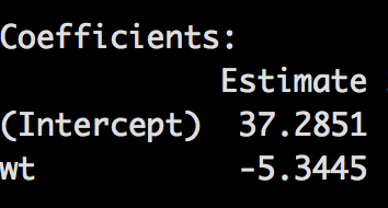
Our first model was predicting mpg using just weight, which looks like this;

intercept + slope*(value) = prediction
=
37.2851 + (-5.3445 )*wt = (???) ̂

So, if it is this easy we should be able to get the same value as the predict function in R by using 2.0 (in thousand pounds) as our weight;

37.2851 + (-5.3445) * 2.0 = 26.5961

Easy huh? Lets do more;

3.0,4.0,9.0

37.2851 + (-5.3445) * 3.0 = 21.2516
37.2851 + (-5.3445) * 4.0 = 15.9071
37.2851 + (-5.3445) * 9.0 = -10.8154

Super easy huh?

So if we start adding more coefficients?

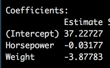
(???) ̂ = 37.22727 + (-3.87783)*Weight + (-0.03177)*Horsepower

Using the same variables from the prior blog post
Horsepower <- c(100,150,200,395)

Weight <- c(2.5,3.5,5.2,5.6)

37.22727 + (-3.87783)*Weight + (-0.03177)*Horsepower

37.22727 + (-3.87783) * 2.5 + (-0.03177) * 100 = 24.35569

37.22727 + (-3.87783) * 3.5 + (-0.03177) * 150 = 18.88936

37.22727 + (-3.87783) * 5.2 + (-0.03177) * 200 = 10.70855

37.22727 + (-3.87783) * 5.6 + (-0.03177) * 395 = 2.962272

If all of our math is correct these will be the same values from the prior blog post.

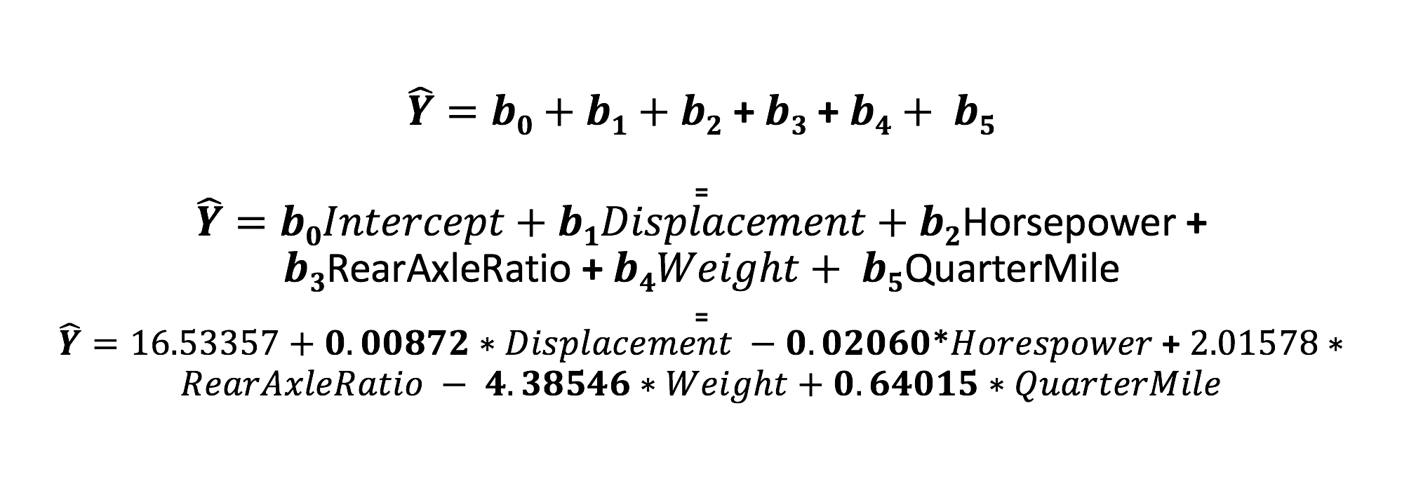
Lets back up for a moment and talk about the formula. Each coefficient can also be called the beta, and as you have learned you can have many, and can be denoted as follows. We did not use these specific values in the prior models, but i think you get the idea. The Y with the carrot symbol is called “y hat” and denotes a prediction estimate since we are using a sample.

“b zero” below will always be the intercept, everything after that is a coefficient, you can see that for 100 variables this could become quire a long formula. Keep in mind that while all of these may not have had a high p-vlaue and were eventually thrown out, they were all quantitative.

To get ready for the next blog we will need to learn a term called an indicator variable, this is what becomes of a qualitative/categorical/factor variable. For this example i will keep the formula short. Lets imagine we have a weight of 2000 pounds, 250 horsepower and a 6 cylinder engine. In the next blog post we will be using cylinder as categorical variable as it descries “which”. R treats factors as indicators, meaning you will have a coefficient for all but the lowest factor in the model, the lowest is assumed to be zero and the result are built from that one, so here is what the model will look like;

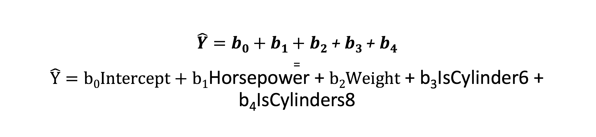
Now we cannot have all the coefficients turned on in this case, because we cannot have a vehicle with 4,6, and 8 cylinders, so we will have to perform the math with some of the indicator variables turned off. SO, if we have the variable, we multiply by 1, if we do not have the variable we multiply by zero.

Our Coefficients;

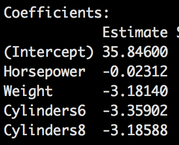
Using our hypothetical car, Our Formula;

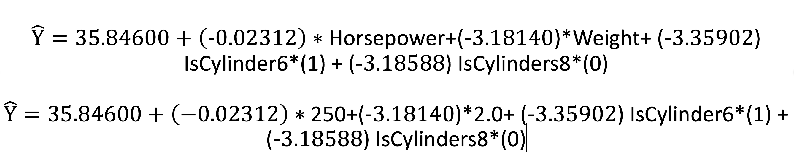
I am hoping, that mathematically that makes sense. In short a 4, 6, and 8 cylinder engine will all have different coefficients and since you can only have a car with one of those choices you must choose just one coefficient to use and turn off the other two you are not using. You will also see these referenced as dummy variables. The next blog will get deeper into this, bu i wanted to introduce the math behind it before we go any farther.