Woo Hoo here we go, in this post we will predict a president, sort of, we are going to do it knowing who the winner is so technically we are cheating. But, the main point is to demonstrate the model not the data. The ISLR has an great section on Logistic Regression, though i thing the data chose was terrible. I would advise walking through it then finding a dataset that has a 0 or 1 outcome. Stock market data for models sucks, i really hate using it and really try to avoid it.

Using the dataset and data engineering from the prior blog post we can start. Or grab the Jupyter Notebook for R from here.

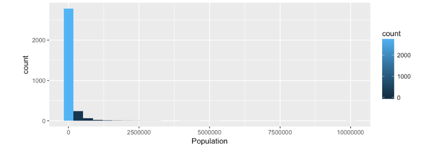
Before we dive deeper lets revisit normal distribution and log using the population data.

ggplot(data=data.Main, aes(Population)) + 
  geom_histogram(aes(fill=..count..))

Looking at the Histogram we can see the data is not normally distributed, almost 3000 counties are piled up in the 0, which we know is not true, but this is what happens when you have an imbalance of values in the data, in this case right skew. The solution is to apply a log normal form of the data by using is log value. log(population).
a

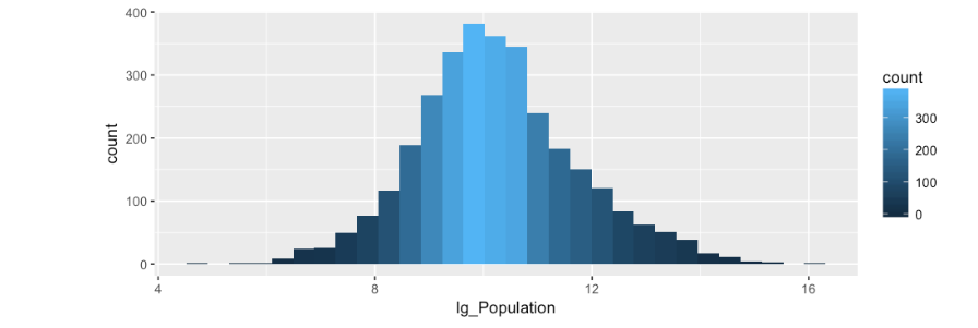
You will notice in the data set provided there is a log form of all the numeric variables already provided with the prefix of lg_.

ggplot(data=data.Main, aes(lg_Population)) + 
  geom_histogram(aes(fill=..count..))

By some voodoo or magic (not really) our population is now normally distributed, which will allow us to use it in a model.

Most of the data is pretty easy to understand by the column names, the only oddity is the RUC_* columns which if you have been keeping up you will notice are already setup as indicator variables. If a county has an RUC=1 only the RUC_1 will have a “1” in it, the other indicator variable columns will be “0”. SO what the heck is RUC? The short answer is, a categorical variable that indicates size range of a county. A value of one indicates a county of greater than 1,000,000 where a value of 9 indicates less than 2500.

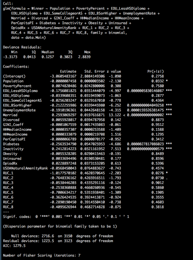
Lets throw everything into the model and see what happens! Noticew we are using glm, and family = binomial, this is R peak for logistic regression.

elect.glm <- glm(Winner~Population + PovertyPercent +
                 EDU_LessHSDiploma + EDU_HSDiploma + EDU_SomeCollegeorAS + EDU_BSorHigher 
                 + UnemploymentRate + Married + Divorced + GINI_Coeff + HHMedianIncome + HHMeanIncome
                 + PerCapitaPI + Diabetes + Inactivity + Obesity + Uninsured + OpiodRx + USDANaturalAmenityRank 
                 + RUC_1 + RUC_2 + RUC_3 + RUC_4 + RUC_5 + RUC_6 + RUC_7 + RUC_8 
                 ,data=data.Main,  family=binomial)
summary(elect.glm)

The worst thing that can possibly happen in your data life is to try and conceive of a model only to find out all of your variables are pretty much useless. Though if you recall from the linear regression posts, the worst thing we can do is dump all the variables into a model as a first step, and second worse thing is to assume they are all bad but 1, population.

The problem is we need to either add the variables one at a time, or remove them one at a time. Lucky for us, stepwise is still a thing for glm.

Lets do a forward stepwise log regression and see what happens.

elect.fwd <- step(glm(Winner~1,data=data.Main,  family=binomial), direction = "forward", 
                  scope=(~Population + PovertyPercent +
                    EDU_LessHSDiploma + EDU_HSDiploma + EDU_SomeCollegeorAS + EDU_BSorHigher 
                    + UnemploymentRate + Married + Divorced + GINI_Coeff + HHMedianIncome + HHMeanIncome
                    + PerCapitaPI + Diabetes + Inactivity + Obesity + Uninsured + OpiodRx + USDANaturalAmenityRank 
                    + RUC_1 + RUC_2 + RUC_3 + RUC_4 + RUC_5 + RUC_6 + RUC_7 + RUC_8 ))


summary(elect.fwd)

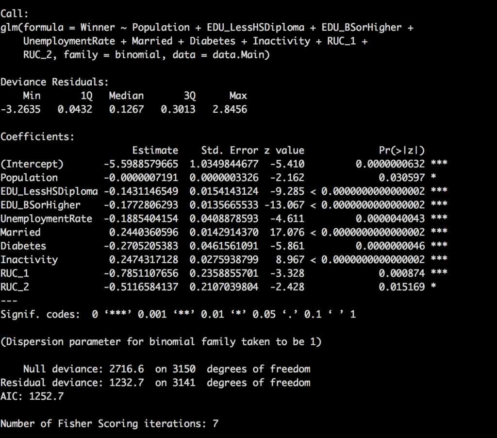
Wowza, we certainly have more than one useful variable now. As discussed in prior posts, RUC_* is a dummy variable, we cannot keep just two of them, its all or nothing.

Lets run the other direction to see of we get the same results.

elect.back <- step(glm(Winner~Population + PovertyPercent +
                        EDU_LessHSDiploma + EDU_HSDiploma + EDU_SomeCollegeorAS + EDU_BSorHigher 
                      + UnemploymentRate + Married + Divorced + GINI_Coeff + HHMedianIncome + HHMeanIncome
                      + PerCapitaPI + Diabetes + Inactivity + Obesity + Uninsured + OpiodRx + USDANaturalAmenityRank 
                      + RUC_1 + RUC_2 + RUC_3 + RUC_4 + RUC_5 + RUC_6 + RUC_7 + RUC_8 
                      ,data=data.Main,  family=binomial), direction = "backward")
summary(elect.back)

Different order, but same values.

Let's see what happens when we use the log versions of the variables? To save some time, lets just slam this into a backward stepwise to see what we get.

elect_lg.glm.back <- step(glm(Winner~lg_Population + lg_PovertyPercent 
                    + lg_EDU_LessHSDiploma + lg_EDU_HSDiploma + lg_EDU_SomeCollegeorAS + lg_EDU_BSorHigher
                    + lg_UnemploymentRate + lg_Married + lg_Divorced + lg_GINI_Coeff + lg_HHMedianIncome + lg_HHMeanIncome
                    + lg_PerCapitaPI + lg_Diabetes + lg_Inactivity + lg_Obesity + lg_Uninsured + lg_OpioidRx
                    + RUC_1 + RUC_2 + RUC_3 + RUC_4 + RUC_5 + RUC_6 + RUC_7 + RUC_8 
                    ,data=data.Main,  family=binomial), direction = "backward")

summary(elect_lg.glm.back)

Notice this time we have 13 variables in the model that were deemed significant, so, changing the variable to log normal did make a pretty big difference. Recall from a prior post about p-value, still true. As a rule we are looking for a p-value of less than 0.05 to claim it is significant.

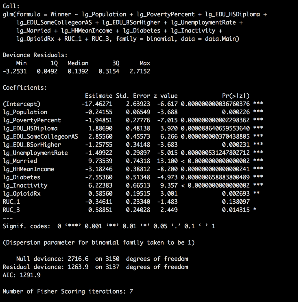
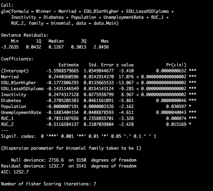
Though the model is looking pretty awesome i am going to remove RUC as it is technically a duplicate of population, in other words, i will correlate to the point it is adding no more value. So lets look at hour new model.

elect_lg.glm <- glm(Winner ~ lg_Population + lg_PovertyPercent + lg_EDU_HSDiploma + 
      lg_EDU_SomeCollegeorAS + lg_EDU_BSorHigher + lg_UnemploymentRate + 
      lg_Married + lg_HHMeanIncome + lg_Diabetes + lg_Inactivity + 
      lg_OpioidRx, family = binomial, data = data.Main)

summary(elect_lg.glm)

Next post we will go through each of the remaining variables and talk about the other data spit out from the model.