From the last post, we have a dataset, now lets do something with it.

To make life easier on you i am providing the data i am using, its already engineered, more could be done, i still have more than one test per vehicle per procedure, but i’m leaving it for now. You can if you want, narrow it down even further by selecting just one test procedure type per vehicle. See last post to get the details on what that means.

So, lets load the data, convert factors.

epaMpg <- read.csv("epaMpg.csv",stringsAsFactors=FALSE)

summary(epaMpg)

epaMpg$Cylinders <- as.factor(epaMpg$Cylinders)
epaMpg$Tested.Transmission.Type.Code <- as.factor(epaMpg$Tested.Transmission.Type.Code)
epaMpg$Gears <- as.factor(epaMpg$Gears)
epaMpg$Test.Procedure.Cd <- as.factor(epaMpg$Test.Procedure.Cd)
epaMpg$Drive.System.Code <- as.factor(epaMpg$Drive.System.Code)
epaMpg$Test.Fuel.Type.Cd <- as.factor(epaMpg$Test.Fuel.Type.Cd)


epaMpg <- epaMpg[!is.na(epaMpg$Cylinders),]

You should have in the neighborhood of 1034 rows if you used my dataset, yours may vary. Next, lets stuff it into a model with abandon and see what we get.

# scipen will just blow out the  scientific notation, i like to see the number. 
options(scipen = 999)

# this should be familiar by now. 
epaMpg.1 <- lm(FuelEcon ~ HorsePower + Cylinders + Tested.Transmission.Type.Code + Gears + Drive.System.Code + Weight + AxleRatio + Test.Procedure.Cd + Test.Fuel.Type.Cd,data=epaMpg)

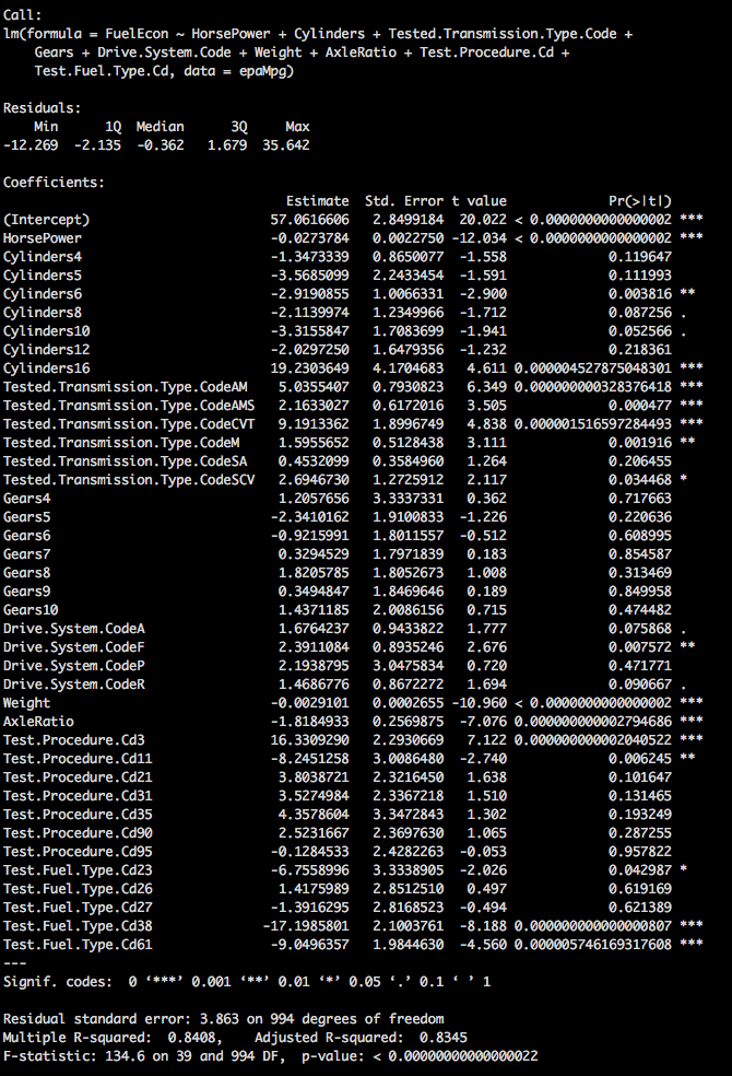
summary(epaMpg.1)

We have a pretty significant model now, lots of data, lots of numbers, Adjusted R² is 83.45% which is not bad at all, Residual standard error at 3.863 is relatively low as it is in units of MPG.

We also have a lot of variables that look like they need to be ditched, so we could go through and drop one, rerun the model check the p-values, drop another, rerun the model check the p-values, drop another rerun the model check the p-values. See a pattern developing there? There is a better way.

So, what do we do? Froward and Backward stepwise regression... You can get a load of useful information on page 207 pf the ISLR, i will let you read all of it. In short, Forward stepwise starts with no predictors and adds the rest one at a time until all of them are in the model. The algorithm will use a combination of R² AIC, BIC and Mallows C(p) to determine which ones to keep. the final best model will be in "epaMpg.fwd1" in this case. Be sure to scroll up through the console to review the output, it is interesting to see what it does to get to the end.

##stepwise regression forward
epaMpg.fwd1 <- step(lm(FuelEcon~1,data=epaMpg), direction = "forward", 
                  scope=(~HorsePower + Cylinders + Tested.Transmission.Type.Code + Gears + Drive.System.Code + Weight + AxleRatio + Test.Procedure.Cd + Test.Fuel.Type.Cd)) 

summary(epaMpg.fwd1)

Surprisingly, forward is not enough, it is possible to run the model in both directions, as in, start with no variables and add one at a time, and start with all variables eliminate the worst one at a time and get different models. For this reason there is also a backward regression.

epaMpg.back1 <- step(lm(FuelEcon ~ HorsePower + Cylinders + Tested.Transmission.Type.Code + Gears + Drive.System.Code + Weight + AxleRatio + Test.Procedure.Cd + Test.Fuel.Type.Cd,data=epaMpg), direction = "backward")
summary(epaMpg.back1)

Well, we have three models, they are all filled with jibber jabber, is there anyway i can compare them without looking at every variable side by side? Yes, yes there is.

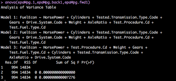
ANOVA, which actually is another statistical learning thing called analysis of variance that will usually tell you the difference in means among groups, but in R, it will also tell you the difference in models.

anova(epaMpg.1,epaMpg.back1,epaMpg.fwd1)

So, what to look for? Lowest RSS, lowest p-value, of all the models this will get you to a starting place to focus in a single model to start working with. In our case, the model i created with all variables and the one generated by the forward stepwise regression as well as the backward stepwise regression all came out to be the same. So, we have a model!

I don't want to get into variable selection cost when dumping all variables into a model and then attempting every variation over every variable, but you can guess its a lot, and its expensive. To give you a place to read up on this, check out page 207 in the ISLR as stated above, it discusses the cost. 2^p number of possible models, p being equal the number of variables, it adds up fast. we have 9 in ours, so 2⁹ models to test if we test everything, but only 512... And as stated in the ISLR forward and backward stepwise only test a subset of that, math is on page 208 of ISLR, i will not be a better person for it, so i am not going to bother diving deep into it and explaining it to you.

Point is, what if i do want to test all 512 variations? There is a package i mentioned couple of posts back that will do this and give us a lot of data, olsrr with the function ols_all_subset()

So, lets try one out! We already have a model created in epaMpg.1, so we will use that one, but remember as it is stated in the variable selection documentation that running this will test 2^p variable combinations, so 20 variables will be 2²⁰ = 1,048,576 combinations. So, when you run ols_all_subset, it will test all variables, so it will be much much slower.

ols <- ols_all_subset(epaMpg.1)
View(ols)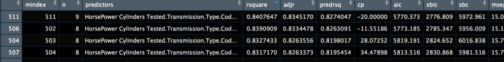

The View() will allow you to view the results in the R console, you can sort and review the data at a minimum you will see that the lowest AIC and the highest R-square is the model we have chose with all variables. The variables tested for each configuration are also listed so you can get an idea of what is best, from this you can create queries to include or exclude criteria if you have a larger dataset.

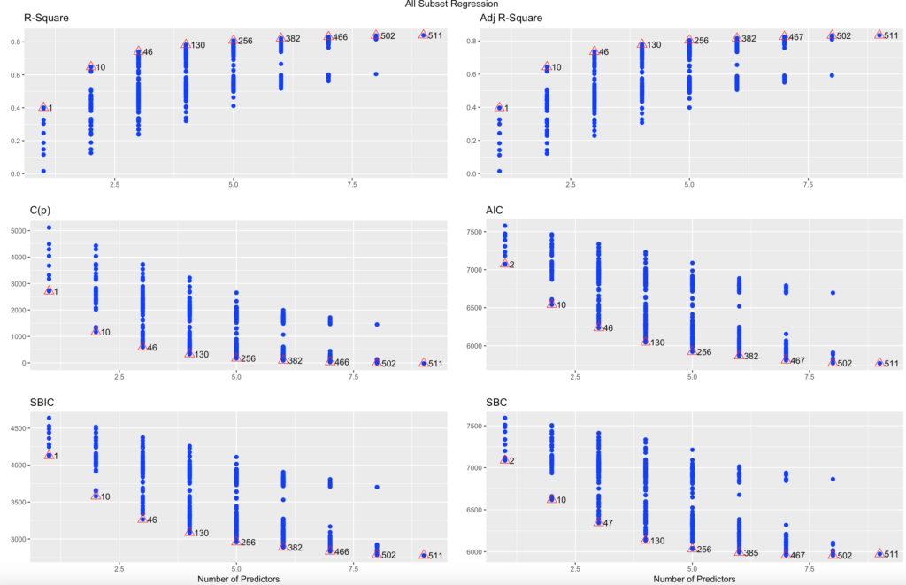
You can also plot ols;

plot(ols)

In my dataset test 511 had the best R-Square, adjusted R-square and the lowest AIC, Lowest Mallows Cp, and lowest BIC. So, must be the best one...?