In the last regression post we added more variables, but not all of them, I was holding back and not telling you why. So far we have been dealing with quantitative variables which ask how many or how much, the next is qualitative or categorical. Categorical usually asks which, and while it may be a number it would not make sense to perform math against it.
SO, what do we have in the data set that is not math friendly and could be considered a category?
Model could be, you cannot add or subtract and does answer the question of which.
Cylinders is, we only have three possible values and does describe a which or what.
VSengine has only two possible values, 0 or 1 indicating straight block engine config or v config.
TransmissionAM has only two possible values, automatic or manual.
Gears is also fixed, only three possible values.
Carburetors is as well, there are 1,2,3,4,6,8 and it would not makes sense to perform any real math opeeration on carb.
Great, so we have identified them, what do we do with them? Easy, tell R they are qualitative.
# picking up where we left off yesterday, i will assume the mtcars is loaded and column names have been changed.
# create factors
ColNames <- c("Cylinders","VSengine","TransmissionAM","Gears","Carburetors")
mtcars[ColNames] <- lapply(mtcars[ColNames], factor)

summary(mtcars)
str(mtcars)
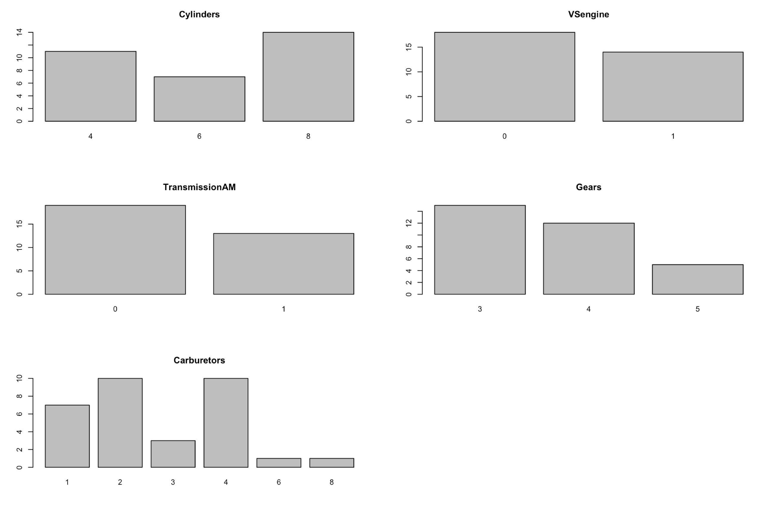
When you run summary and str you will see that the column types are now factors and indicate the number of levels. Summary will show the number of rows for each level. You will also notice that when you run base R graphics commands against factors you get slightly different behavior. Using plot below you will get a histogram.
par(mfrow=c(3,2))
plot(mtcars$Cylinders,main="Cylinders")
plot(mtcars$VSengine,main="VSengine")
plot(mtcars$TransmissionAM,main="TransmissionAM")
plot(mtcars$Gears,main="Gears")
plot(mtcars$Carburetors,main="Carburetors")
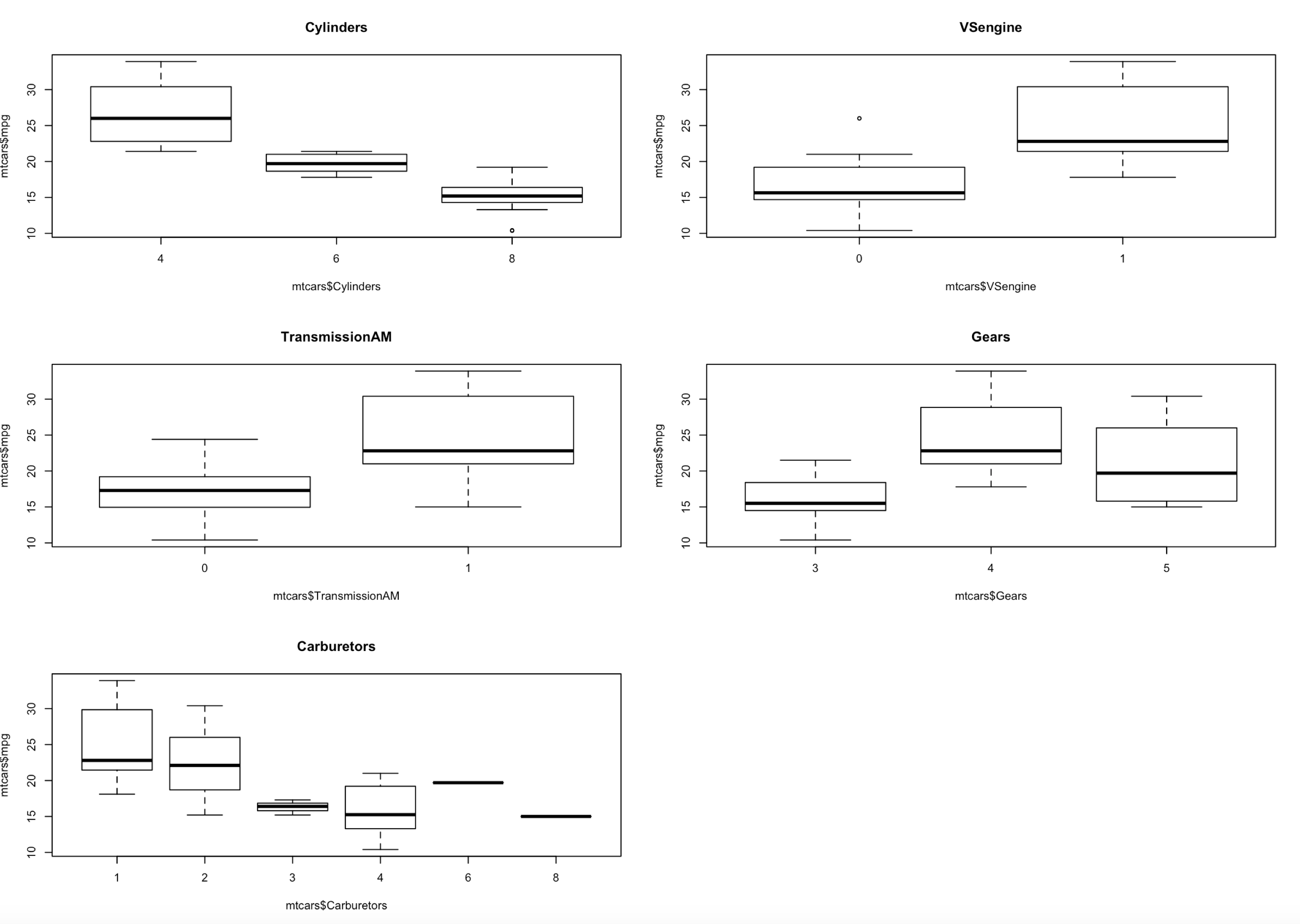
For more plotting fun when you add the y axis to plot you will get a boxlot on a factor vs. a scatterplot. I did do a write up on boxlot here.
par(mfrow=c(3,2))
plot(mtcars$mpg ~ mtcars$Cylinders, main="Cylinders")
plot(mtcars$mpg ~ mtcars$VSengine,main="VSengine")
plot(mtcars$mpg ~ mtcars$TransmissionAM,main="TransmissionAM")
plot(mtcars$mpg ~ mtcars$Gears,main="Gears")
plot(mtcars$mpg ~ mtcars$Carburetors,main="Carburetors")
In linear regression a factor is not treated the same as a quantitative variable, a factor actually becomes a thing called an indicator variable. As in, the coefficient for a 4 cylinder vs. a 6 cylinder vs. 8 cylinder can all be different but for a single calculation only one of them will be used. Also, each factor will show as an individual coefficient.
Take a look at the coefficients below;
mtcars.5 <- lm(mpg ~ Horsepower + Weight + Cylinders, data=mtcars)
summary(mtcars.5)
When a factor is added to the model each value in the factor will get a coefficient except the lowest, that one will have a coefficient of zero, so no need to actually add it and you can assume that if the value of the cylinder what we are trying to predict is 4, then none of the indicators will be turned on, or used in other words.
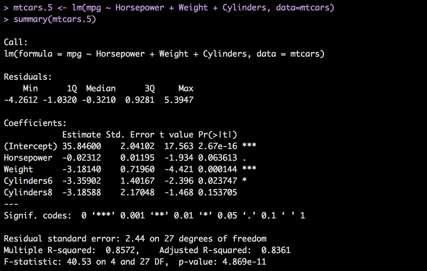
We have to perform the same diligence with a categorical variable as we do with a quantitative variable. While they may look funny in the model, in some packages when you ready to do a prediction we will have to create a column for every indicator, but not R. We will still need to look at the p-value to see if it is adding any value. However, one thing you must consider, if you keep one indicator variable from a factor you have to keep them all. For instance In the model mtcars.5 that was created above, Cylinders6 has a low p-value, but Cylinders8 has a p-value above .05 which we would typically throw out, but we cannot throw just one of them out, we have to keep them all or throw all of them out.
To show you how messy this can become lets add all of the categorical variables to the model.
mtcars.6 <- lm(mpg ~ Horsepower + Weight + Cylinders + VSengine + TransmissionAM + Gears + Carburetors, data=mtcars)
summary(mtcars.6)
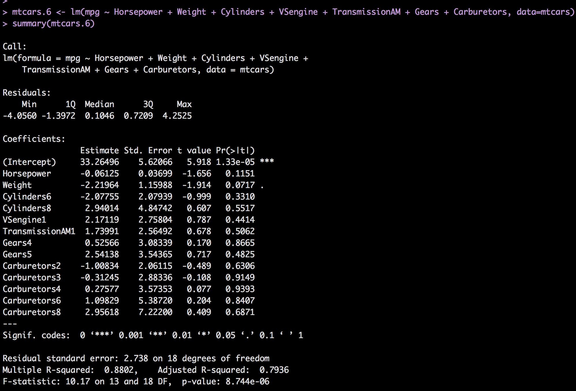
You will notice the model got a whole lot busier, and all the p-values are really bad except for weight! Even Horsepower is above .05 now. The very next blog post will get into how to deal with a model when you have this much variability, and we already know that adding and subtracting variables will improve then degrade the model depending on the order we do it. There is a better way! For now, i am going to jump to the end and show you the best model we can arrive at, then do a prediction.
First whats the least annoying model?
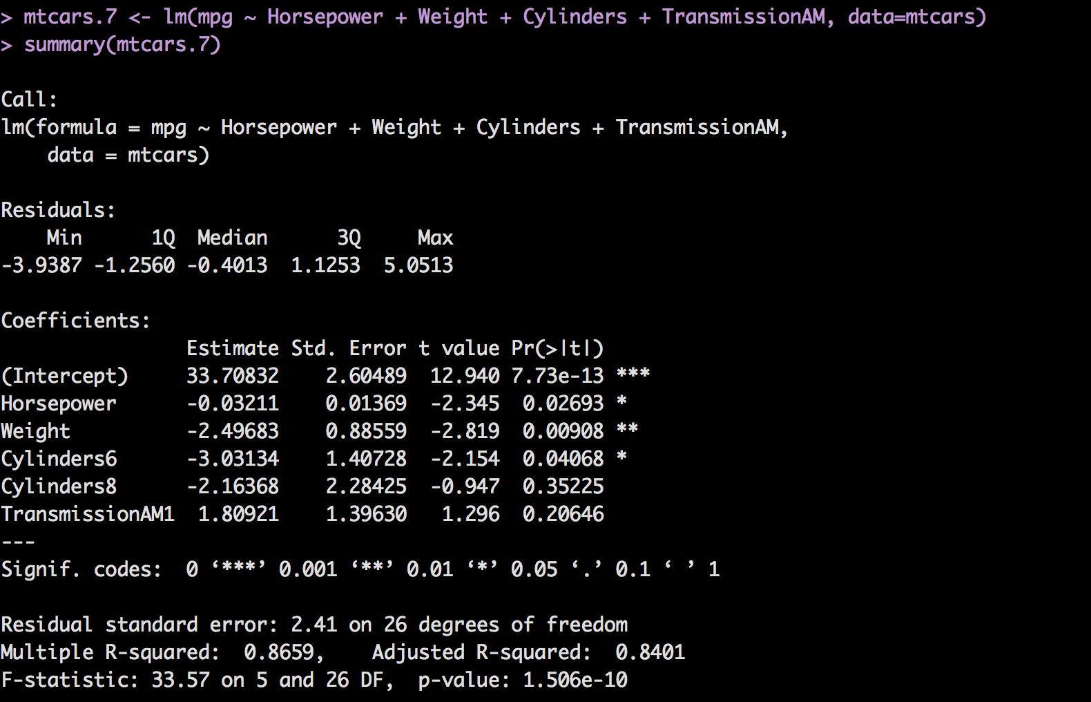
mtcars.7 <- lm(mpg ~ Horsepower + Weight + Cylinders + TransmissionAM, data=mtcars)
summary(mtcars.7)
Recall what i said about indicator variables, if one is good and one is bad you will have to decide to keep all of it or none of it. In this case we are keeping Cylinders. TransmissioNAM1, has a high p-value but if we remove it, something else will spike up, so its a balance of least worst. Adjsuted R-square is high, p-value for model is low, f-statistic is far from one. Residual standard error of 2.41 relative to intercept is pretty low, which is good.
Now, for the prediction. This is where indicator variables become annoying in most software packages. R however, is extremely friendly and will handle the pivot and indicator variable for you behind the scene. Packages like SPSS will require you to create the indicator variable manually if a factor is present. Our data frame going in will look like this;
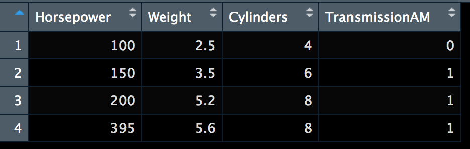
Horsepower <- c(100,150,200,395)
Weight <- c(2.5,3.5,5.2,5.6)
Cylinders <- as.factor(c(4,6,8,8))
TransmissionAM <- as.factor(c(0,1,1,1))
newcars = data.frame(Horsepower,Weight,Cylinders,TransmissionAM)
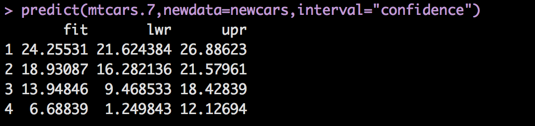
predict(mtcars.7,newdata=newcars,interval="confidence")
And of course the output;
The true test as always, much like any software is to test it over and over again. Make sure the training data you use represents the real world data that the model will be used to predict.
To give you an example the last in the newcars dataframe, 395 horse power, 5600 pounds, 8 cylinder engine, and automatic transmission has a predicted mpg of 6.7 but may be as low as 1.2mpg and as high as 12.1mpg. I can tell you that is not correct, that is my current vehicle, and gets around 15-20mpg depending on highway or city. But the model was trained with a small set of data form 1974, it cannot be used for anything outside of that time frame and car characteristics.
Next we will look at how to deal with figuring out a model with dozens of variables...