You were warned! If you have ever sat in on a single data science talk you probably learned that the data engineering phase of a project will take 80% of your time. This is an anecdotal number, but my experience to date seems to reenforce this number. On average it will take about 80% of whatever time you have to perform the data engineering tasks. This blog is going to likely prove that, though you will not have had to do the actual work, just copy and paste the code and run it. You will however get an idea of the pain in the ass you are in for.

I am going to approach this post and the scripts exactly the way i came to the dataset, so i will remove rows, then learn something new and remove some more rows or maybe add them back. I could simply put the data engineering at the top, and not explain anything but that is not how the world will work. The second, third, forth, one hundredth time you do this you will have the scripts and knowledge. With any new dataset, curiosity and exploration will make the process of modeling much easier.

Here is the thing; A SQL Pro can typically do this work in T-SQL lickety-split, in R or Python you may be learning as you go. I always seem to know what i want to accomplish, but R frequently refuses to bend to my will. I will show you more than one way to do something, if i can find a solution using a tidyverse solution i will, but as of now i find dplyr syntax unfriendly and cumbersome. I look forward to the day that i find it as useful as the folks pushing it down my throat as the end all to data engineering. But, come June of this year i will be going head first full time Python, that day may have to wait.

In continuing with the MPG problem i will use a 2018 EPA data set. Here is the csv i am using. Here is the link to the EPA website where more info can be found. This is the link to the pdf containing column descriptions and values, the data dictionary if you will. It appears that it has not been updated since the 90’s, so i am not sure if i have the wrong file or they really have not updated it since the 90’s. You can derive some of the column values and meanings, but not all, you may need to do a bit of spelunking. I do have a copy of the data file i am using on my github site, just in case the file they publish gets updated and the wacky values you are about to see get fixed. I already have a pretty good idea of what columns to use since i want to keep this as close to the mtcars problem as possible, but you will soon find out there is more than one answer to MPG.

# If you do not want to download the file, you can read it directly from the source into a dataframe.
# epa <- read.csv("https://www.epa.gov/sites/production/files/2017-10/18tstcar.csv",stringsAsFactors=FALSE)

#If the above does not work get it from my github site, 
# https://raw.githubusercontent.com/sqlshep/SQLShepBlog/master/data/18tstcar.csv

# or
# Set working dir if you download this locally
getwd()
setwd("/Users/AwesomeUser/data")

epa <- read.csv("18tstcar.csv",stringsAsFactors=FALSE)

Never be afraid to change column names while you are learning if you need to, however, if you are working with others or have a standard data dictionary for a production system be very careful, this is also a very good way to piss everyone off. I will change the names in this dataframe to come closer to what we were using in the last few mtcars examples.

# there are several ways to rename columns, here are three ways to do it, 
# choose your fav and stick with it

names(epa)[12] <-paste("Cylinders")
names(epa)[46] <-paste("FuelEcon")

colnames(epa)[colnames(epa)=="X..of.Gears"] <- "Gears"
colnames(epa)[colnames(epa)=="Axle.Ratio"] <- "AxleRatio"

epa <- dplyr::rename(epa, HorsePower = "Rated.Horsepower")
epa <- dplyr::rename(epa, Weight = "Equivalent.Test.Weight..lbs..")
epa <- dplyr::rename(epa, Model = "Represented.Test.Veh.Model")

The exploration part of the project is very important, look at everything

# you do not need all of these right now, but you will later. 
library(dplyr)
library(ggplot2)
library(GGally)

ggplot(epa,aes(FuelEcon,Weight))+
  geom_point()

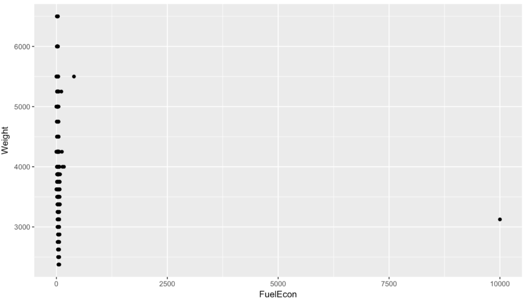
In case you are wondering when the data engineering shit show begins, its now. We have weight and mpg and a car that claims to get 10,000 mpg. My best advice is to treat it like a game, find and conquer weird data. Now you have to determine what vehicle gets 10,000 mpg and is it cool enough for you to buy? No, i mean should you remove the row, fix the value, leave the value, and find out why you have a value that is so wrong. Bad data and missing data is something that has to be dealt with very strategically.

The following will produce any row with mpg > 9000 and the three rows for the Chevy Sonic, make sure you can isolate it.

filter(epa,   FuelEcon > 9000)

epa[epa$Test.Vehicle.ID == "184HV863DA" ,]
epa[epa$Test.Vehicle.ID == "184HV863DA" ,c("Represented.Test.Veh.Make","Model","Test.Vehicle.ID","FuelEcon")]

According to Fuel Economy website the mpg should be 30 combined, so we can fix it by script or fix the original source. But, much like SQL be careful. In addition to wiping out you did not mean to, once you make a modification it needs to be reproducible. If you need to go through 25 steps to modify a dataset do you want to do it one row at a time in excel or text editor? A better way is to script everything so it is easily reproducible and fast. In a given day on the data engineering work i will reload then main data file and run all of my modifications several times a day to make sure everything is working and reproducible. Don't assume you will remember everything if you need to start over, write it down, write it down in scripts.

Notice the total rows in the dataframe, and how many NA's (no value) we have. Then overwrite the dataframe OR or create a new one with everything less than 9999 mpg.

summary(epa$FuelEcon)

#  > summary(epa$FuelEcon)
#  Min.  1st Qu.   Median     Mean  3rd Qu.     Max.     NA's 
#  0.00    24.40    30.90    35.86    40.30 10000.00       12 

NROW(epa)

#> NROW(epa)
# [1] 3509

epa <- (filter(epa, FuelEcon < 9999))

Notice below we have 13 less rows, the 12 NA's are gone and the 10,000mg car is gone. In my case this is fine, i am okay with deleting the 12 NA rows, but in the real world you may need to decide how to handle them? Why is there data missing? Do you need to leave the rows and fix the missing data issue either with imputation or actually getting the data? What method should you use to do this? In my case the first problem was bad data, so why do i have a car with 10,000 mpg? All of these need to be addressed by the data domain expert. In the end the answer may be to delete the row, but at some point this too will become a problem, i have worked with customers where 98% of the data had to be thrown out for a variety of reasons. It is possible throw out so much data that you no longer have a project, and this is a real problem you will encounter some day.

summary(epa$FuelEcon)

#  > summary(epa$FuelEcon)
#  Min. 1st Qu.  Median    Mean 3rd Qu.    Max. 
#  0.00   24.40   30.85   33.01   40.28  395.40 

NROW(epa)
# > NROW(epa)
# [1] 3496

Lets look at our plot again.

ggplot(epa,aes(FuelEcon,Weight))+
  geom_point()

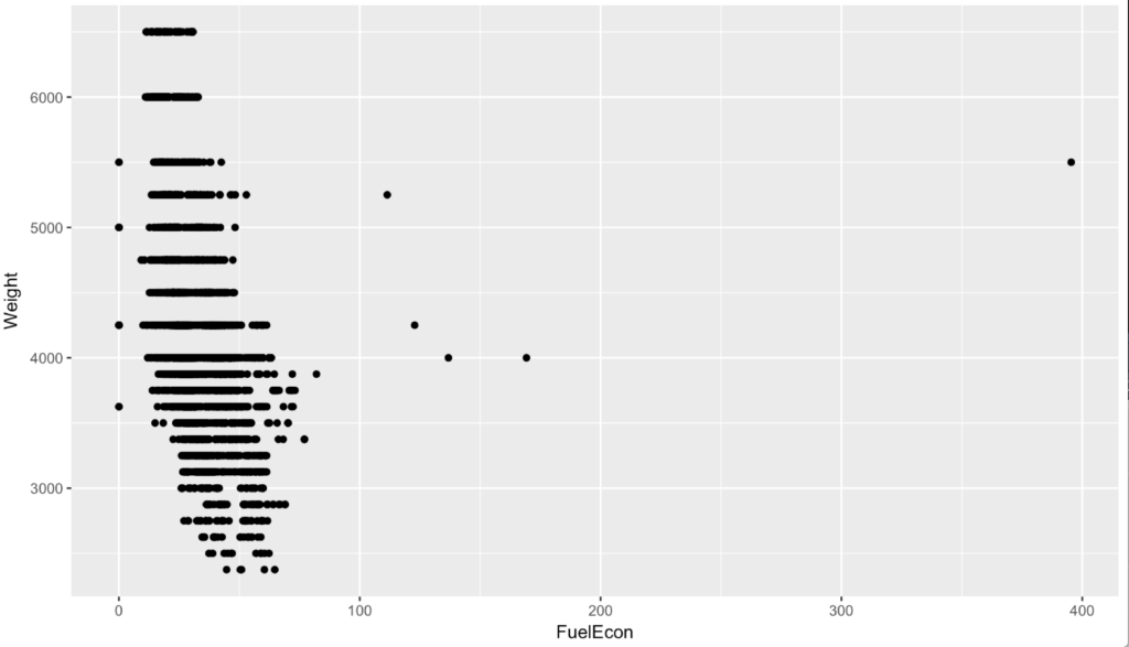
Well, its better but now i have what are clear outliers and one in the 400 mpg range. Now, i once had a 3000 pound diesel car and it got no where near 400 mpg, so i am going to assume this is either bad data or a Tesla. Lets add some labels to just the outliers.

ggplot(epa, aes(FuelEcon,Weight)) +
  geom_point() +
  geom_text(data=subset(epa, FuelEcon > 90),aes(FuelEcon,Weight,label=Model), vjust=-.5, hjust=.10)

# you can also use the following code to find more outliers, though technically, 
# an outlier is > 2 standard deviations away from the mean, see if you can calculate that. 

#filter(epa, FuelEcon > 100)
#epa[epa$FuelEcon > 100 ,c("Represented.Test.Veh.Make","Model","Test.Vehicle.ID","FuelEcon")]

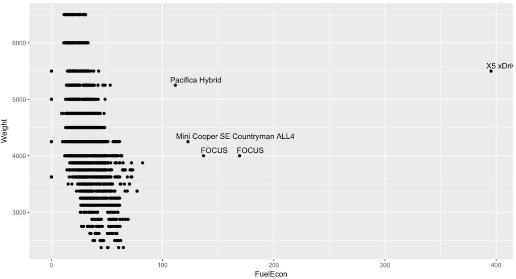
Nope its a BMW X5 xDrive40e, and its not all electric, its hybrid and it does not get 395, its more around 24 - 56 mpg depending on "mode", so, bad data. From looking at the file and the codes in the file, it does not appear we have a way to identify a hybrid or all electric car with a binary. However, the EPA requires tests that are unique to electrics and hybrids. In the "Test Procedure Description" column you will find "Charge Depleting Highway" and "Charge Depleting UDDS" values, as well as "Test Fuel Type Description" of Electricity, though, a hybrid may also use tier 2 gasoline, so it is not mutually exclusive, meaning it can be tested for charge depletion and run on gasoline too. So in the interest of a petrol only mpg data set i think i will delete the electric and hybrid cars. Keep in mind, these could be kept in and used as an indicator/dummy variable to. If you were to used Hybrid as a variable it would likely have a pretty significant coefficient. It may be fun to take just the hybrids and create a separate model completely. Never be afraid to do that if necessary, ensemble models are all the rage.

The Cruze is not hybrid but the data set claims 77mpg, which doing a little research even the best Diesel Cruze reports are around 55mpg and there is anecdotal evidence of hyper mile-ing to get up to 70, but i am sure the EPA did not do that. So, what do we do? I am leaving the cruze, because for me to be critical of one and not all would be unfair. I am going to remove the electrics and hybrids and see where we end up.

View(filter(epa,   Test.Procedure.Description == "Charge Depleting Highway" | Test.Procedure.Description == "Charge Depleting UDDS"))

epa <- filter(epa,   Test.Procedure.Description != "Charge Depleting Highway" & Test.Procedure.Description != "Charge Depleting UDDS")


ggplot(epa,aes(FuelEcon,Weight))+
  geom_point()

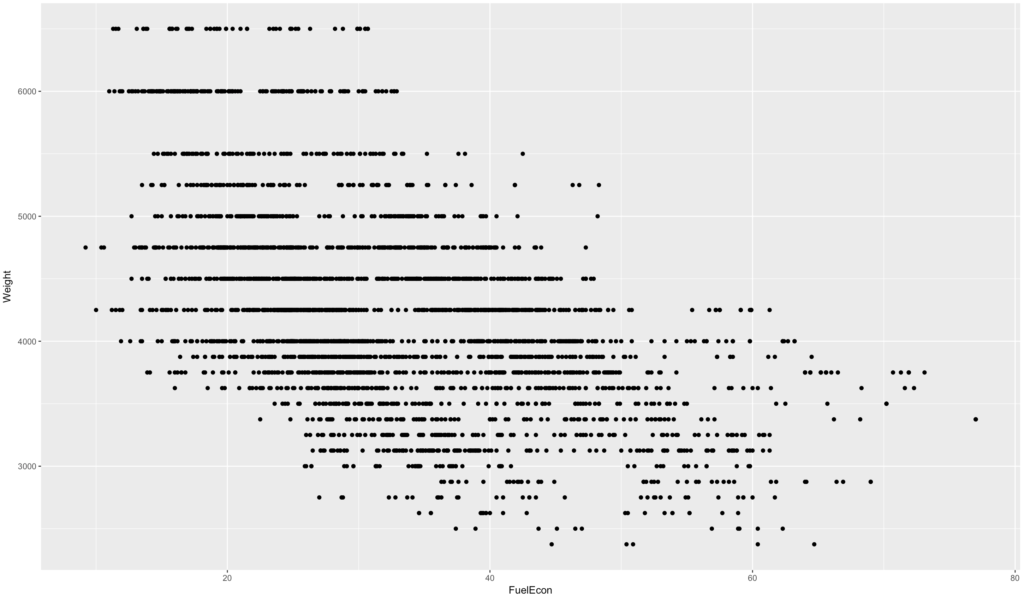
This looks much nicer, and gets our dataset in a little better shape.

Notice the weights this time, they all seem to be rather perfect. The weight of a vehicle is very dynamic from vehicle to vehicle. You can run summary(as.factor(epa$Weight)) and see that all of the vehicles were rounded to within 250lbs of actual weight. Which is interesting because this opens the possibility of using this as a factor or an indicator variable in the regression model. But, we will deal with weight shortly.

Lets take a closer look at a couple of cars.

View(filter(epa,   Represented.Test.Veh.Make == "BENTLEY" & Model == "Continental GT" ))

You will notice that we have multiple rows for each car, if you have not realized that look a little closer. Each row represents a different EPA test, and there are at least 5 test run on each vehicle. You can learn more about the process of EPA testing here. There are a couple of ways to approach this, you can leave all of the tests in, make the testa a factor and add it to the model so that you have to indicate which test you want predictions from, which is what i will do. You could also split out the test into different models, i may do that later to see if it makes a difference in model accuracy.

The following will display the number of cars in each test, it is clearly imbalanced.

table(epa$Test.Procedure.Description)

I want to be cognizant of the data i am removing, that being said this is still a toy training set just for fun. We may need to remove rows since a higher number of rows of one vehicle type can skew the model toward that type of vehicle performance. For instance, if i have 100 vehicles in the training data set that get 15mpg and 10 that get 40mpg, and that does not represent real world, the model will be heavily influenced by the 100 vehicles that get 15 mpg thus skewing all predictions. I would want the model to be as accurate as possible for the 40mpg as it is for the 15mpg, now, maybe the data will exist to help differentiate that, like and 8 cylinder engine vs. a three cylinder, and a weight of 8000 pounds vs 2000 pounds, but then again maybe not... In this dataset with Vehicle.ID == "53XECSE012" the only significant difference is the fuel, E85 Ethanol and gasoline. SO what would be the appropriate thing to do? The Suburban has 58 rows, and the Civic, Vehicle.ID == "EGAA1M" has 40 rows. In the real world, this may need to be dealt with.

The following code will show the highest number of tests per vehicle, though you can also see that there is a minor configuration change for each test though perhaps not so significant that it should result in a training row for a model...? This is where the data domain expert is useful in helping decide if the vehicles with minor changes should be included or excluded.

k<-table(epa$Test.Vehicle.ID)
head(sort(k,decreasing = TRUE))

View(filter(epa, epa$Test.Vehicle.ID == "53XECSE012"))

k1<-filter(epa, epa$Test.Vehicle.ID == "53XECSE012")
table(k1$Model,k1$Test.Fuel.Type.Description)
table(k1$Test.Fuel.Type.Description,round(k1$FuelEcon))

I do want to remove the police interceptors.

# Police 
View(filter(epa, epa$Police...Emergency.Vehicle. == "Y"))
table(epa$Police...Emergency.Vehicle.)
epa <- filter(epa,epa$Police...Emergency.Vehicle. != "Y" )

Well, that was awesome, we dropped a few rows but still ahve a long way to go. If you have browsed the data you will see that there are still alot of test for a single vehicle that seem very very close to each other, what wee need is a good old fashion distinct to get the almost duplicates out. Lucky for us there is one, distinct from dplyr will allow us to specify the columns we want distinct tested against while still allowing us to present the entire row. As a SQL guy all i can say is where have you been all my life.

# Review distinct 
View(distinct(epa,Vehicle.Manufacturer.Name
              ,Veh.Mfr.Code
              ,Represented.Test.Veh.Make
              ,Model
              ,Test.Vehicle.ID
              ,Test.Veh.Displacement..L.
              ,Drive.System.Description
              ,AxelRatio
              ,Weight
              ,Test.Fuel.Type.Cd
              , .keep_all = TRUE))

# Reload dataframe with less values. 
epa <- (distinct(epa,Vehicle.Manufacturer.Name
              ,Veh.Mfr.Code
              ,Represented.Test.Veh.Make
              ,Model
              ,Test.Vehicle.ID
              ,Test.Veh.Displacement..L.
              ,Drive.System.Description
              ,AxelRatio
              ,Weight
              ,Test.Fuel.Type.Cd
              , .keep_all = TRUE) )

My dataset is now down to 1/3 of what it was, recall what i said about throwing all of your data out, we won't get that far but i think you see how easy it can happen.

At some point, or any point we could start throwing columns that will not be part of the training set. Remember that most of the columns are emissions test results and all we are looking for is mpg. Now what may be fun later on is to take this same dataset and predict what our emissions could be based on a configuration. So far we have kept the entire 67 variables, lets start dumping them.

So, what do we want to keep?

While it may not matter at this point, but, i am going to create a dew data frame to work with, epaMpg.

# trim down the columns for the mdel training set 
View(epa[c(4,5,10,11,12,14,15,16,18,22,23,34,35,36,37,46)])

epaMpg <- epa[c(4,5,10,11,12,14,15,16,18,22,23,34,35,36,37,46)]

names(epaMpg)

Lets convert the columns to factors that need to be factors.

epaMpg$Cylinders <- as.factor(epaMpg$Cylinders)
epaMpg$Tested.Transmission.Type.Code <- as.factor(epaMpg$Tested.Transmission.Type.Code)
epaMpg$Gears <- as.factor(epaMpg$Gears)
epaMpg$Test.Procedure.Cd <- as.factor(epaMpg$Test.Procedure.Cd)
epaMpg$Drive.System.Code <- as.factor(epaMpg$Drive.System.Code)
epaMpg$Test.Fuel.Type.Cd <- as.factor(epaMpg$Test.Fuel.Type.Cd)

For fun, if you want to do something somewhat silly, run ggpairs against the dataset and review the results, notice the difference between factors and quantitative columns.

ggpairs(epaMpg[c(3:6,14)])
ggpairs(epaMpg[c(8:12,14)])

This is one version of the data engineering, this process is iterative, and can go on for days, even for a small dataset. A question to answer is essential, and a data domain expert is essential to help make sense of the data.