In Logistic Regression 3 we created a model, quite blindly i might add. What do i mean by that? I spent a lot of time getting the single data file ready and had thrown out about 50 variables that you never had to worry about. If you are feeling froggy you can go to the census and every government website to create your own file with 100+ variables. But, sometimes its more fun to tale your data and slam it into a model and see what happens.
What still needs done is to look for colliniearity in the data, in the last post i removed the RUC variables form the model since the will change exactly with the population, the only thing they may add value to is if i wanted to use a factor for population vs. the actual value.
If you are more interested in Python i have created a notebook using the same dataset but with the python solution here.
So, where we left off. You will find a new Jupyter notebook here with the same name as the blog, feel free to download it and the prior ones.
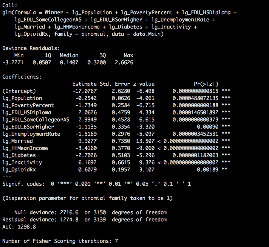
elect_lg.glm <- glm(Winner ~ lg_Population + lg_PovertyPercent + lg_EDU_HSDiploma +
      lg_EDU_SomeCollegeorAS + lg_EDU_BSorHigher + lg_UnemploymentRate +
      lg_Married + lg_HHMeanIncome + lg_Diabetes + lg_Inactivity +
      lg_OpioidRx, family = binomial, data = data.Main)

summary(elect_lg.glm)
Notice all of hour p-values are less than .05 which is what we truly desire in life, what we do not know is if any of the remaining variables are collinear, so how mighty we figure that out? vif() THe generic rule of thumb for the vif is an variable that has a value greater than two is suspect. Seriously, thats it, its suspect, suspect of what you may ask, suspect of being collinear.
x<-vif(elect_lg.glm)
data.frame(x)
vif(elect.glm) > 2
x[vif(elect.glm) > 2]
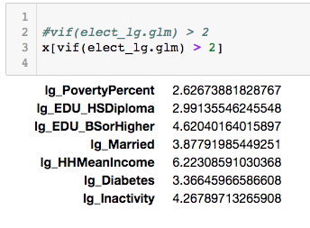
There are a few that are above two, but quite frankly it still a pretty useless definition. SO lets dig a little deeper.
Lets create a vector of column names that ahve a value of greater than 2 and run them through ggpairs and see what some scatterplots and correlations look like.
cols = c("Winner",names(x[vif(elect_lg.glm) > 2]))
print(cols)
#This will take a minute or two
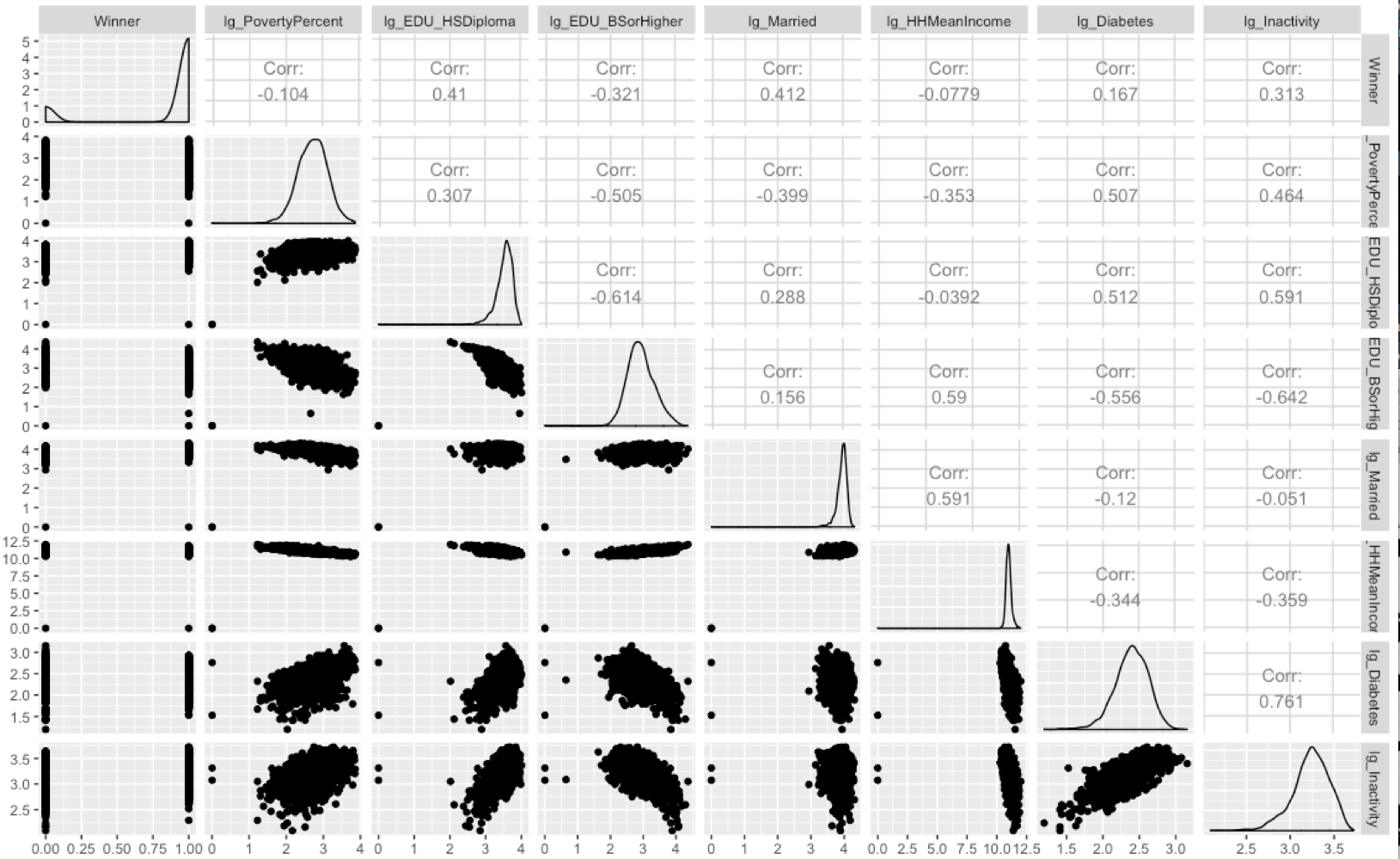
ggpairs(data=data.Main,columns=cols)
You will have to zoom in to get a good look at this, but what we can see that a few of theses have a positive correlation, Inactivity, EDU_BSorHigher HHMeanIncome have a pretty high vif, and looking at the correlations also have pretty high values.
Lets unpack this; EDU_HSDiploma indicates the percentage of the county that completed high school but went no further and correlates to Winner with a .41 which means i positively correlates indicating counties with a high EDU_HSDiploma percentage typically vte at a higher rate for Trump. Also, counties that have a higher percentage of Married couples also correlated at .412. While not are main interest you can see that there is a correlation in counties with inactivity(lg_Inactivity) and diabetes (lg_Diabetes), not really a shocker that those two correlate.
So the question becomes if you have variables that are correlated do you leave them in or take them out? This is where the causation, correlation, and spurious correlation come into play. You have to think about it and make a decisions. Me? I am going to leave everything in, as is.
I am not going to go crazy on this next section of model evaluation, logistic regression is an annoying one that determine a rock solid model really is a bit of voodoo. What we can do after our data engineering, and correlation test is perform a Hosmer-Lemeshow goodness of fit test which will spit out a guess what? A P-Value, but wait, i am going to blow your mind, the p-value in this case needs to be above .05. ?
Great article on "The Hosmer-Lemeshow goodness of fit test for logistic regression", skip past the math notation if it freaks you out, the R code is there too.
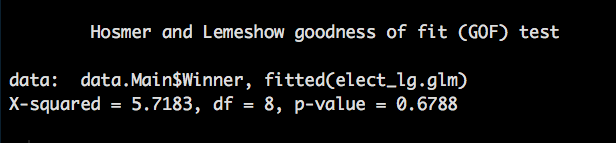
Lets see how our model is doing with Hosmer-Lemeshow
install.packages("ResourceSelection")
library(ResourceSelection)

hoslem.test(elect_lg.glm$y, fitted(elect_lg.glm), g=10)
A p-value of .6788 is not disappointing at all considering we are looking for anything above .05. However, one thing Hosmer-Lemeshow does not take into account is overfitting, so that is still a concern.
The last item to do in our evaluation is to check the confusion matrix.
elect.probs = predict(elect_lg.glm, type="response")
elect.probs[1:10]
data.Hold <- data.Main
elect.pred=rep("Trump",3151)
elect.pred[elect.probs < .5] = "Hillary"
data.Hold$Winner[data.Hold$Winner == '1'] ="Trump"
data.Hold$Winner[data.Hold$Winner == '0'] ="Hillary"
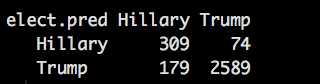
table(elect.pred,data.Hold$Winner)
If you ahve forgotten what a confusion matrix is,
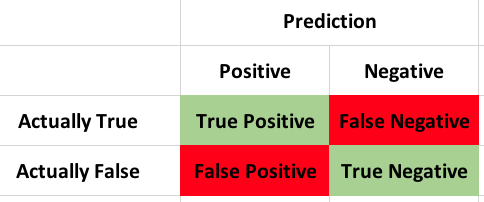
What we are interested in are the TP and TN this gives our accuracy of the model (309+2589)/3151 = 0.919708 accuracy. Little creepy huh? It would appear that base don this data the model was able to predict the outcome of the election with 92% certainty, keeping in mind that we trained and tested on the same dataset, so technically it should be a nearly perfect fit. In the next post i will pullout a train and test set and see if it is still so good...