Lets try and bring simple linear regression together before i move on to multiple. We started with a question, can we predict miles per gallon using weight of a vehicle? We looked at a scatter plot and saw a bit of linearity. We created a model and looked at the residuals and determined they are for he most part demonstrating constant variance and we looked at a histogram of the residuals and it is demonstrating enough normal distribution to move forward. I know, i’m not sounding very convincing am i? Its a small dataset and its for learning, having some values that are out in left and right field but are actually useful so i can demonstrate some other points later in this post.

Lets review the output form summary(mtcasr.1).

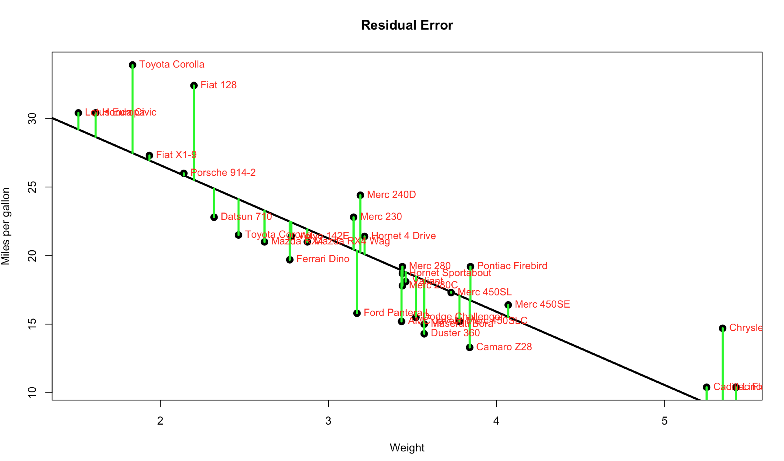
Residuals: not much to see here, you need to look at these in a scatter plot or histogram.

Coefficients: Intercept is mpg in this case, the estimate is where the line crosses the y axis at Zero. mtcars$wt is the slope of the line.

Standard error: Imagine this as the confidence interval of the estimate, it is all so the expected error +/-. When we do the prediction this may make more sense.

T-Value: is the estimate/standard error the farther from 1 the better.

p-value: Usually <.05 is used and what you are looking for, but it may be .01 or .001.

Residual Standard Error: Is the average amount the prediction will deviate form the linear regression line.

R-Squared: How well does the model do at predicting mpg based on wt. 1 Is perfect fit, 0 is no fit. Be weary of 1, or.99 theat may be overfit which is bad.

F-Statistic: should be far from 1, but how far depends on the units. This is a good measure of the entire model and useful for comparing one model to another.

p-value: P-Value for the entire model, again <.05 is the generic goal, also useful when comparing one model to another.

C’MON PREDICT SOMETHING ALREADY!


Let me show the minimum in case you are starting here. Create the model and store the results in mtcars.1, run a summary.

When you create the model, make sure you pass in the dataframe using “data=”. I occasionally get lazy and create the model by directly referencing the columns and not using lm, this will work by the prediction will thrown warnings like “Warning message:
‘newdata’ had 1 row but variables found have 32 rows” and the result set will be the entire dataframe which is not what you want.

data(mtcars)

#  Right way
mtcars.1 <- lm(mpg ~ wt, data=mtcars)

## This is the wrong way... 
## mtcars.1 <- lm(mtcars$mpg ~ mtcars$wt)

Since we only have one explanatory variable we can pass in a list, in this case a list of just one value, 2000 pounds, which is 2 in our dataset.

predict(mtcars.1,list(wt=c(2.0)))

Okay! So this tells us that based on the data the model was trained with a vehicle that ways 2000 pounds is expected to get about 26.6mpg based on the 32 1974 vehicles we have. WHich if you go back and look at the dataset you will see that is somewhere in the 2140 and 1935 pounds. Works as expected.

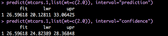
So, what else can we do? interval="prediction", or interval="confidence". These are very close but still different, the definition of each must be precise, and it trips me up.

Confidence: The confidence interval also called the mean interval asks what is the mpg of a car at a specific weight. You will notice we had a tighter response band between lower and upper in the output of confidence vs prediction. What you see in the numbers is within the 95% confidence interval that the mpg will be between 24.82389 28.36848 based on the model.

Prediction: While similar, the main difference is the standard error is taken into consideration as part of the calculation which allows for a wider band or upper and lower range of values.

You can read more about this prediction and confidence here. Sometimes i'm happy to say the software does it for me.

predict(mtcars.1,list(wt=c(2.0)), interval="prediction")
predict(mtcars.1,list(wt=c(2.0)), interval="confidence")

That was fun, now what? Lets add a few more data points to the prediction. We now have 2000, 3000,4000, and 9000 pounds using the confidence so we can see an upper and lower range.

predict(mtcars.1,list(wt=c(2.0,3.0,4.0,9.0)), interval="confidence")

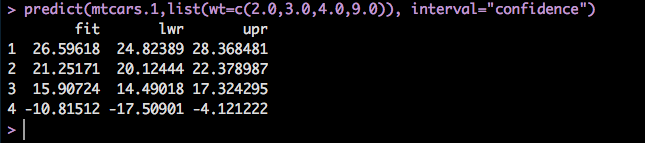
If we take a look at the mtcars dataframe the mpgs do not look out of place for 2000,3000,4000 pounds, however the 9000 pounds is -10 mpg. I once drove a vehicle that got 7 mpg, luckily it was someone elses problem to pay for the gas. But, -10 is not a scale that makes any sense. SO what happened?

Remember that the model can only provide an accurate estimate for data it has been trained with, the heaviest vehicle in the dataset is 5424 pounds and there is no data to determine what 9000 pounds would be for mpg. Aside from that also recall that in linear regression it is running a straight line through the dataset that will provide a mean of zero residual errors based on the data you provide it. Looking again at the scatter plot below, imagine the line goes off into infinity through the y axis on the upper left, and through the x axis on the bottom right. The prediction is where the weight intercepts the linear regression line.

If we expand the x and y axis; Notice where the orange(2000 pounds), yellow (3000 pounds) and green(4000 pounds) line cross the linear regression line, this is the estimate of mpg provided by the predict R command. Visually it makes sense that it can only make an accurate prediction for the data it was trained with, so when we attempt to predict 9000 pounds indicated in blue, it won't work. This is a very important point for all data science prediction tasks, what was the model trained with?

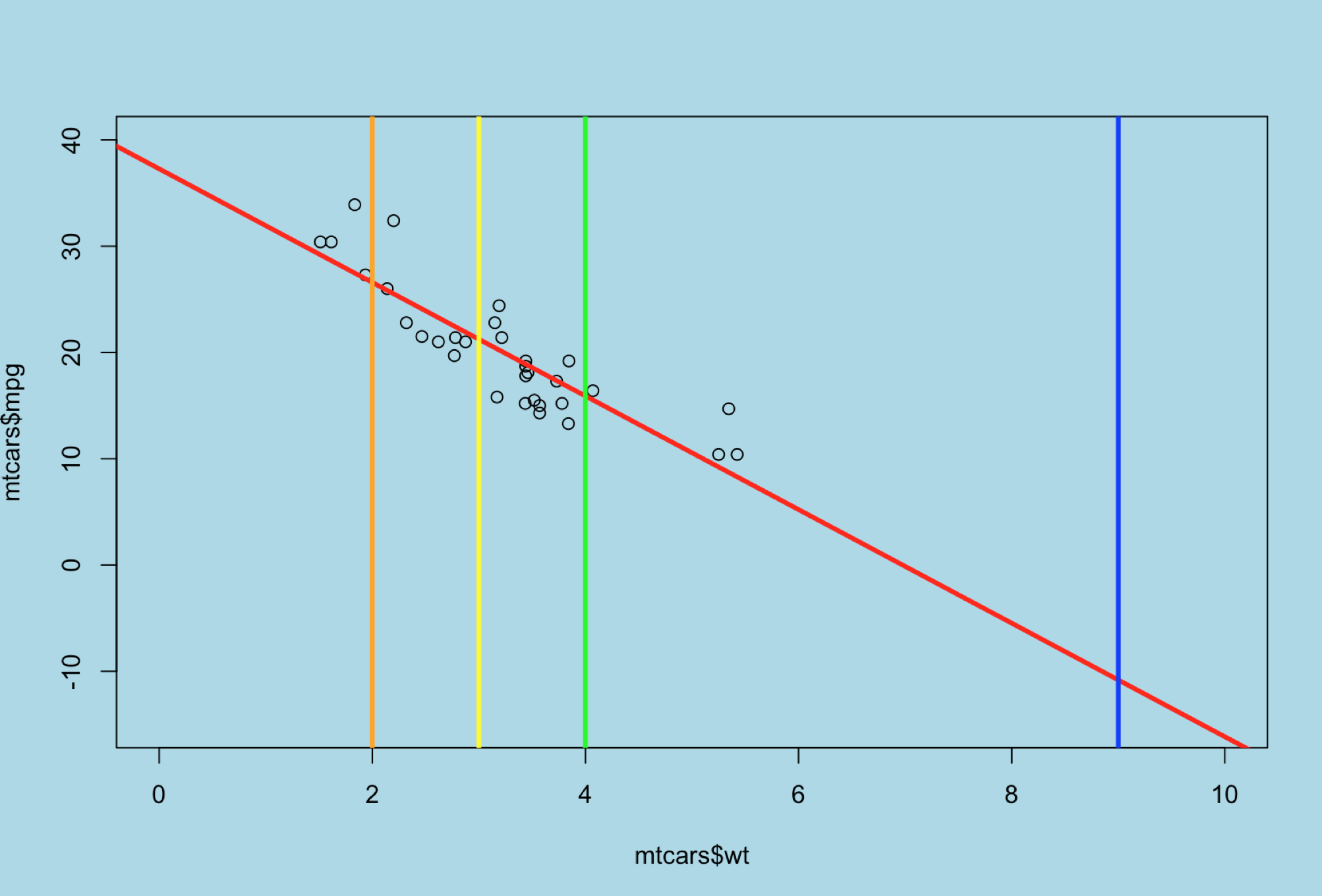
If you want to recreate the above scatterplot...

par(bg = 'lightblue')
plot(mpg~wt,data=mtcars,
     ylim=c(-15,40),
     xlim=(c(0,10))
)
abline(lm(mtcars$mpg ~ mtcars$wt), col="red",lwd=3)
abline(v=2.0, col="orange",lwd=3)
abline(v=3.0, col="yellow",lwd=3)
abline(v=4.0, col="green",lwd=3)
abline(v=9.0, col="blue",lwd=3)

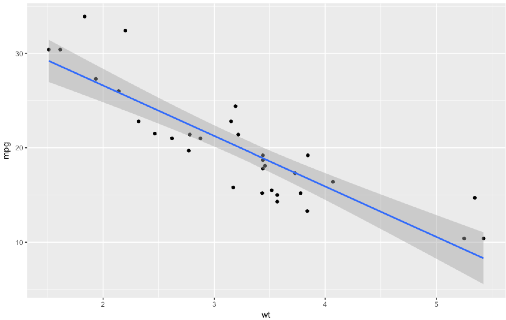
One final note, you can use ggplot to provide confidence intervals in an scatterplot. When i start the next post on multiple linear regression i will move to ggplot vs. base r graphics. Code follows;

library(ggplot2)

ggplot(mtcars, aes(x=wt, y=mpg)) + 
  geom_point() + 
  geom_smooth(method=lm)

You have to admit, ggplot does produce a more attractive graphic.