This post was certainly not meant to be next, but here it is. I am working on a project that may very well take me a year to complete maybe longer depending on demands. I am also taking this blog into python which was not meant to happen for a while as i would like to get every R post in this blog mirrored with python as well.

But, the problem first, to be fair this could have been done in R, i just happen to be taking some python dev classes at the moment. The problem, i have a document called House Resolution 1, H.R.1, if you have been on the planet and in the US while the 115th congress was in session you probably heard of it, its the tax act. I wanted to see if anything can be discovered from this bill, longer term i will be looking every piece of legislation from the 115th congress, but one thing at a time. This is the discovery phase, and for me the tool discovery phase as well.

My tools; i do everything in the Spyder IDE, because its awesome, and i try to stay in Anaconda 3. Once things are working nicely i move everything into a Jupyter notebook, and then sometimes a blog as i will probably forget where everything is on my machine.

I just copied HR1 down to my machine, from the link above, just save it as a text file. The process i used to get to the end is not perfect, but it works, and i am sure when i learn more i will teak a bit, and i will say the plots output is friendlier in a notebook, due to some weird behaviors of Spyder and plot sizing. You can grab my notebook from github at the bottom of this post.

To start, lets do our imports, similar to R loading packages and libraries.

import nltk
import os
import string

import matplotlib.pyplot as plt

from nltk.tokenize import RegexpTokenizer
from collections import Counter

nltk.download("stopwords")
nltk.download("punkt")

This is just loading up a list stopwords we will need later, stop words are considered junk words to natural language processing, as you can imagine depending on the doc you are parsing you may have a very different set of words, medical vs. legal vs. engineering. I did add a few to the list, some unusual things that shoed up in the document.

stop_words = nltk.corpus.stopwords.words("english") + list(string.punctuation) \
+ list(string.ascii_lowercase) + list(string.ascii_uppercase) + list(string.digits) \
+ list(['--']+["''"]+["``"]+[".."]+["..."]+["ii"]+["iii"]+["iv"]+["'s"])

print(stop_words)

type(stop_words)

Assuming you have copied the HR1 or whatever do you want to di this down to your machine, the following will read it from the hard drive as a string object, convert the entire doc to lower case, then replace all of the ` with nothing, there are a lot of them in legislation for some reason.

# set working directory and verify
os.chdir("/Users/Me/HR1")
os.getcwd()

# set a pointer and read the file into HR1
a = open("HR1.txt") 
HR1 = a.read()

# Set the entire file to lower case
HR1 = HR1.lower()

# Replace the ' with nothing
HR1 =  HR1.replace("`","")

Tokenize is a weird little thing, complicated way of saying tear my string apart into a bazillion individual strings based on spaces or punctuation. Its still a list, but instead of a list with one string, its a list with n strings, in my case 104,563 strings.

HR1_token = nltk.word_tokenize(HR1)

The following will remove the stop words from my list. After this runs my number of strings will drop to 40,631.

hr1_filter = [w for w in HR1_token if not w in stop_words]

Next we run a counter function to basically count the word left over. You will see we have 3371 unique values, though when you peek you will see this includes numbers and section headings, not terribly meaningful umless one number shows up a lot, like the year maybe.

hr1_counter = Counter(hr1_filter)

Sort the remaining words by count, we are getting ready to graph them.

sorted_word_counts = sorted(list(hr1_counter.values()), reverse=True)

Language processing is new to me so this will probably be a lot more in the weeks and months to come, but here is the idea; if the curve is a relatively flat diagonal this indicates that the words are somewhat evenly distributed, meaning there is no hyper focused central topic in the document, if there is a peak, that should indicate a focused topic. I did expect this to be a bit more focused since it is tax legislation.

plt.loglog(sorted_word_counts)
plt.ylabel("Freq")
plt.xlabel("Word Rank");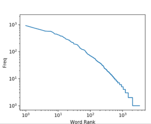

Histogram is super boring, not sure what the point is, but here you go.

plt.hist(sorted_word_counts, bins=50);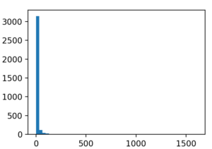

This one is better, using log normal will even out the distribution a little bit, but this is still just eye candy, distribution of words.

plt.hist(sorted_word_counts, bins=50, log=True);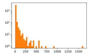

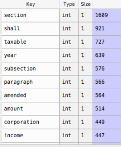
Looking at the top words is somewhat more useful vs. the natural log in a plot…

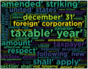
This is where the word cloud can come in, though truthfully, this is just more eye candy, i seriously doubt any executive decision has been made from a word cloud, though if they have i might want to work there, be an easy job, etch and sketch pictures for the boss.

The following may take many seconds to run, the size of 12×12 is a pretty chunky visual to assemble, so if it goes a really long time and bothers you set the width and height to 4 each, that will speed it up, though small.

from wordcloud import WordCloud

width = 12
height = 12
plt.figure(figsize=(width, height))
#text = 'all your base are belong to us all of your base base base'
wordcloud = WordCloud(font_path='/Library/Fonts/Gotham-Bold.otf',width=1800,height=1400).generate(str(hr1_filter))
plt.imshow(wordcloud)
plt.axis("off")
plt.show()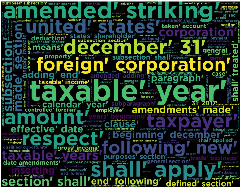

The Python Notebook can be found here, through the awesomeness of github, you can even view it there too.