Category Archives: choropleth

R Markdown

Published / by shep2010

This is a slight diversion into a tool built into R called R Markdown, and Shiny will be coming up in a few days. Why is this important? It gives you a living document you can add text and r scripts to to produce just the output from R. I wrote my Stats grad project using just R Markdown and saved it to a PDF, no Word or open office tools.

Its a mix of HTML and R, so if you know a tiny bit about HTML programing you will be fine, otherwise, use the R Markdown Cheat sheet and Reference Guide which i just annoyingly found out existed…

I am going to give you a full R Markdown document to get you started.

Create a new R Markdown file;

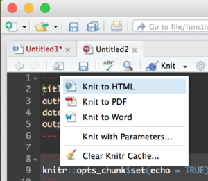
Then Run it by selecting the “Knit” drop down in the middle left of the toolbar and selecting Knit to HTML.

This will create an html document that you can open in a browser, it comes with some default mtcars data just so you can see some output. Try out some R commands and doodle around a bit before starting the code below. This is the file data file we will be using, US-Education.csv It contains just the 2010-2014 educational attainment estimates per count in the US.

In the code books below i will put in each section of the R Markdown and discuss it, each R code block can me moved to r console to be run.

The first section Is the title that will show up on the top of the doc, copy this into the markdown file and run it by itself. I am using an html style tag as i want some of the plots to be two columns across.

You will also see the first R command in an “R” block identified by ““`{r} and terminated with ““`”. Feel free to remove options and change options to see what happens.

Notice below the style tag is wrong, when you copy it out you will need to put the “<" back in from of the style tag. If i format it correctly wordpress takes it as an internal style tag to this post.


---
title: "Educational Attainment by County"

output: html_document
---

style>
  .col2 {
    columns: 2 200px;         /* number of columns and width in pixels*/
    -webkit-columns: 2 200px; /* chrome, safari */
    -moz-columns: 2 200px;    /* firefox */
     line-height: 2em;
     font-size: 10pt;

  }

/style>

```{r setup, include=FALSE}
knitr::opts_chunk$set(echo = FALSE,warning=FALSE)

#require is the fancy version of install package/library
require(choroplethr)

```

This will be the next section in the markup, load a dataframe for each of the four educational attainment categories.


```{r one}

#Load data
 setwd("/data/")
 usa <- read.csv("US-Education.csv",stringsAsFactors=FALSE)

#Seperate data for choropleth 
 lessHighSchool <- subset(usa[c("FIPS.Code","Percent.of.adults.with.less.than.a.high.school.diploma..2010.2014")],FIPS.Code >0)
 
highSchool <- subset(usa[c("FIPS.Code","Percent.of.adults.with.a.high.school.diploma.only..2010.2014")],FIPS.Code >0) 
 
someCollege <- subset(usa[c("FIPS.Code","Percent.of.adults.completing.some.college.or.associate.s.degree..2010.2014")],FIPS.Code >0)
 
college <- subset(usa[c("FIPS.Code","Percent.of.adults.with.a.bachelor.s.degree.or.higher..2010.2014")],FIPS.Code >0)

#rename columns for Choropleth
 
 colnames(lessHighSchool)[which(colnames(lessHighSchool) == 'FIPS.Code')] <- 'region'
 
 colnames(lessHighSchool)[which(colnames(lessHighSchool) == 'Percent.of.adults.with.less.than.a.high.school.diploma..2010.2014')] <- 'value'

# 
# or
#
 names(highSchool) <-c("region","value")
 names(someCollege) <-c("region","value")
 names(college) <-c("region","value")
 
 
```

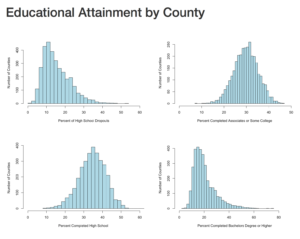
The next section will create four histograms of the college attainment by category. Notice the distribution of the data, normal distribution, right skew, left skew, bimodal? We will discuss them next blog.

Notice for the next section i have the "div" without the left "<", be sure to put those back.


div class="col2">

```{r Histogram 1}
 hist(lessHighSchool$value,xlim=c(0,60),breaks=30, xlab = "Percent of High School Dropouts", ylab="Number of Counties",main="",col="lightblue")


 hist(highSchool$value,xlim=c(0,60),breaks=30, xlab = "Percent Completed High School ", ylab="Number of Counties",main="",col="lightblue")
 
```
 
 
```{r Histogram 2}

 hist(someCollege$value,xlim=c(0,50),breaks=30, xlab = "Percent Completed Associates or Some College ", ylab="Number of Counties",main="",col="lightblue")
 
 hist(college$value,xlim=c(0,90),breaks=30, xlab = "Percent Completed Bachelors Degree or Higher ", ylab="Number of Counties",main="",col="lightblue")


```

/div>


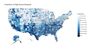
The next section is the choropleth, for the high school dropouts, notice the R chunk parameters to size the plot area.


```{r two, fig.width=9, fig.height=5, fig.align='right'}


 county_choropleth(lessHighSchool,
                  
                   title = "Proportion of High School Dropouts",
                   legend="Proportion",
                   num_colors=9)
 
```

There are three more choropleths that you will have to do on your own! you have the data, and the syntax. If you have trouble with this, the red file i used is here Education.rmd

In the end, you should have a histogram looking like this;

And if you make it to the first choropleth, Percentage that did not complete high school;

Visualization, The gateway drug II

Published / by shep2010

In the last blog you were able to get a dataset with county and population data to display on a US map and zoom in on a state, and maybe even a county if you went exploring.  In this demo we will be using the same choroplethr package but this time we will be using external data.  Specifically, we will focus on one state, and check out the education level per county for one state.

The data is hosted by the USDA Economic Research Division,  under Data Products / County-level Data Sets.  What will be demonstrated is the proportion of the population who have completed college, the datasets “completed some college”, “completed high school”, and “did not complete high school” are also available on the USDA site.

For this effort, You can grab the data off my GitHub site or the data is at the bottom of this blog post, copy it out into a plain text file. Make sure you change the name of the file in the script below, or make sure the file you create is “Edu_CollegeDegree-FL.csv”.

Generally speaking when you start working with GIS data of any sort you enter a whole new world of acronyms and in many cases mathematics to deal with the craziness.  The package we are using eliminates almost all of this for quick and dirty graphics via the choroplethr package.  The county choropleth takes two values, the first is the region which must be the FIPS code for that county.  If you happen to be working with states, then the FIPS state code must be used for region.  To make it somewhat easier, the first two digits of the county FIPS code is the state code, the remainder is the county code for the data we will be working with.

So let’s get to it;

Install and load the choroplethr package


install.packages("choroplethr")
library(choroplethr)

Use the setwd() to set the local working directory, getwd() will display what the current R working directory.


setwd("/Users/Data")
getwd()


Read.csv will read in a comma delimited file. “<-“ is the assignment operator, much like using the “=”. The “=” can be used as well. Which to assignment operator to use is a bit if a religious argument in the R community, i will stay out of it.


# read a csv file from my working directory 
edu.CollegeDegree <- read.csv("Edu_CollegeDegree-FL.csv")


View() will open a new tab and display the contents of the data frame.


View(edu.CollegeDegree) 

str() will display the structure of the data frame, essentially what are the data types of the data frame


str(edu.CollegeDegree)

Looking at the structure of the dataframe we can see that the counties imported as Factors, for this task it will not matter as i will not need the county names, but in the future it may become a problem. To nip this we will reimport using stringsAsFactors option of read.csv we will get into factors later, but for now we don't need them.


edu.CollegeDegree <- read.csv("Edu_CollegeDegree-FL.csv",stringsAsFactors=FALSE)

#Recheck our structure 
str(edu.CollegeDegree)


Now the region/county name is a character however, the there is actually more data in the file than we need. While we only have 68 counties, we have more columns/variables than we need. The only year i am interested in is the CollegeDegree2010.2014 so there are several ways to remove the unwanted columns.

The following is actually using index to include only columns 1,2,3,8 much like using column numbers in SQL vs the actual column name, this can bite you in the butt if the order or number of columns change though not required for this import, header=True never hurts. You only need to run one of the following commands below, but you can see two ways to reference columns.


edu.CollegeDegree <- read.csv("Edu_CollegeDegree-FL.csv", header=TRUE,stringsAsFactors=FALSE)[c(1,2,3,8)]

# or Use the colun names

edu.CollegeDegree <- read.csv("Edu_CollegeDegree-FL.csv", header=TRUE,stringsAsFactors=FALSE)[c("FIPS","region","X2013RuralUrbanCode","CollegeDegree2010.2014")]

#Lets check str again
str(edu.CollegeDegree)

Using summary() we can start reviewing the data from statistical perspective. The CollegeDegree2010.2014 variable, we can see the county with the lowest proportion of college graduates is .075, or 7.5% of the population of that county the max value is 44.3%. The average across all counties is 20.32% that have completed college.


summary(edu.CollegeDegree)

Looking at the data we can see that we have a FIPS code, and the only other column we are interested in for mapping is CollegeDegree2010.2014, so lets create a dataframe with just what we need.


View(edu.CollegeDegree)

# the follwoing will create a datafram with just the FIPS and percentage of college grads
flCollege <- edu.CollegeDegree[c(1,4)]

# Alternatively, you can use the column names vs. the positions. Probably smarter ;-) 
flCollege <- edu.CollegeDegree[c("FIPS","CollegeDegree2010.2014")]

# the following will create a dataframe with just the FIPS and percentage of college grads

flCollege 

But, from reading the help file on county_choropleth, it requires that only two variables(columns) be passed in, region, and value. Region must be a FIPS code so, we need to rename the columns using colnames().


colnames(flCollege)[which(colnames(flCollege) == 'FIPS')] <- 'region'
colnames(flCollege)[which(colnames(flCollege) == 'CollegeDegree2010.2014')] <- 'value'

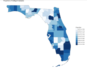
So, lets map it!

Since we are only using Florida, set the state_zoom, it will work without the zoom but you will get many warnings. You will also notice a warning that 12000 is not mappable. Looking at the data you will see that 12000 is the entire state of Florida.


county_choropleth(flCollege,
                  title = "Proportion of College Graduates ",
                  legend="Proportion",
                  num_colors=9,
                  state_zoom="florida")

For your next task, go find a different state and a different data set from the USDA or anywhere else for that matter and create your own map. Beware of the "value", that must be an integer, sometimes these get imported as character if there is a comma in the number. This may be a good opportunity for you to learn about gsub and as.numeric, it would look something like the following command. Florida is the dataframe, and MedianIncome is the column.


florida$MedianIncome <- as.numeric(gsub(",", "",florida$MedianIncome))


USDA Economic Research Division Sample Data


FIPS,region,2013RuralUrbanCode,CollegeDegree1970,CollegeDegree1980,CollegeDegree1990,CollegeDegree2000,CollegeDegree2010-2014
12001,"Alachua, FL",2,0.231,0.294,0.346,0.387,0.408
12003,"Baker, FL",1,0.036,0.057,0.057,0.082,0.109
12005,"Bay, FL",3,0.092,0.132,0.157,0.177,0.216
12007,"Bradford, FL",6,0.045,0.076,0.081,0.084,0.104
12009,"Brevard, FL",2,0.151,0.171,0.204,0.236,0.267
12011,"Broward, FL",1,0.097,0.151,0.188,0.245,0.302
12013,"Calhoun, FL",6,0.06,0.069,0.082,0.077,0.092
12015,"Charlotte, FL",3,0.088,0.128,0.134,0.176,0.209
12017,"Citrus, FL",3,0.06,0.071,0.104,0.132,0.168
12019,"Clay, FL",1,0.098,0.168,0.179,0.201,0.236
12021,"Collier, FL",2,0.155,0.185,0.223,0.279,0.323
12023,"Columbia, FL",4,0.083,0.093,0.11,0.109,0.141
12027,"DeSoto, FL",6,0.048,0.082,0.076,0.084,0.099
12029,"Dixie, FL",6,0.056,0.049,0.062,0.068,0.075
12031,"Duval, FL",1,0.089,0.14,0.184,0.219,0.265
12033,"Escambia, FL",2,0.092,0.141,0.182,0.21,0.239
12035,"Flagler, FL",2,0.047,0.137,0.173,0.212,0.234
12000,Florida,0,0.103,0.149,0.183,0.223,0.268
12037,"Franklin, FL",6,0.046,0.09,0.124,0.124,0.16
12039,"Gadsden, FL",2,0.046,0.086,0.112,0.129,0.163
12041,"Gilchrist, FL",2,0.027,0.071,0.074,0.094,0.11
12043,"Glades, FL",6,0.031,0.078,0.071,0.098,0.103
12045,"Gulf, FL",3,0.057,0.068,0.092,0.101,0.147
12047,"Hamilton, FL",6,0.055,0.059,0.07,0.073,0.108
12049,"Hardee, FL",6,0.045,0.074,0.086,0.084,0.1
12051,"Hendry, FL",4,0.076,0.076,0.1,0.082,0.106
12053,"Hernando, FL",1,0.061,0.086,0.097,0.127,0.157
12055,"Highlands, FL",3,0.081,0.097,0.109,0.136,0.159
12057,"Hillsborough, FL",1,0.086,0.145,0.202,0.251,0.298
12059,"Holmes, FL",6,0.034,0.06,0.074,0.088,0.109
12061,"Indian River, FL",3,0.107,0.155,0.191,0.231,0.267
12063,"Jackson, FL",6,0.064,0.081,0.109,0.128,0.142
12065,"Jefferson, FL",2,0.061,0.113,0.147,0.169,0.178
12067,"Lafayette, FL",9,0.048,0.085,0.052,0.072,0.116
12069,"Lake, FL",1,0.091,0.126,0.127,0.166,0.21
12071,"Lee, FL",2,0.099,0.133,0.164,0.211,0.253
12073,"Leon, FL",2,0.241,0.32,0.371,0.417,0.443
12075,"Levy, FL",6,0.051,0.078,0.083,0.106,0.105
12077,"Liberty, FL",8,0.058,0.08,0.073,0.074,0.131
12079,"Madison, FL",6,0.07,0.083,0.097,0.102,0.104
12081,"Manatee, FL",2,0.096,0.124,0.155,0.208,0.275
12083,"Marion, FL",2,0.074,0.096,0.115,0.137,0.172
12085,"Martin, FL",2,0.079,0.16,0.203,0.263,0.312
12086,"Miami-Dade, FL",1,0.108,0.168,0.188,0.217,0.264
12087,"Monroe, FL",4,0.091,0.159,0.203,0.255,0.297
12089,"Nassau, FL",1,0.049,0.091,0.125,0.189,0.23
12091,"Okaloosa, FL",3,0.132,0.166,0.21,0.242,0.281
12093,"Okeechobee, FL",4,0.047,0.057,0.098,0.089,0.107
12095,"Orange, FL",1,0.116,0.157,0.212,0.261,0.306
12097,"Osceola, FL",1,0.067,0.092,0.112,0.157,0.178
12099,"Palm Beach, FL",1,0.119,0.171,0.221,0.277,0.328
12101,"Pasco, FL",1,0.049,0.068,0.091,0.131,0.211
12103,"Pinellas, FL",1,0.1,0.146,0.185,0.229,0.283
12105,"Polk, FL",2,0.088,0.114,0.129,0.149,0.186
12107,"Putnam, FL",4,0.062,0.081,0.083,0.094,0.116
12113,"Santa Rosa, FL",2,0.098,0.144,0.186,0.229,0.265
12115,"Sarasota, FL",2,0.142,0.177,0.219,0.274,0.311
12117,"Seminole, FL",1,0.094,0.195,0.263,0.31,0.35
12109,"St. Johns, FL",1,0.085,0.144,0.236,0.331,0.414
12111,"St. Lucie, FL",2,0.081,0.109,0.131,0.151,0.19
12119,"Sumter, FL",3,0.047,0.07,0.078,0.122,0.264
12121,"Suwannee, FL",6,0.056,0.065,0.082,0.105,0.119
12123,"Taylor, FL",6,0.064,0.086,0.098,0.089,0.1
12125,"Union, FL",6,0.033,0.059,0.079,0.075,0.086
12127,"Volusia, FL",2,0.107,0.13,0.148,0.176,0.213
12129,"Wakulla, FL",2,0.018,0.084,0.101,0.157,0.172
12131,"Walton, FL",3,0.067,0.096,0.119,0.162,0.251
12133,"Washington, FL",6,0.04,0.063,0.074,0.092,0.114

Visualization, The Gateway Drug

Published / by shep2010

Visualization is said to be the gateway drug to statistics. In an effort to get you all hooked, I am going to spend some time on visualization. Its fun (I promise), i expect that after you see how easy some visuals are in R you will be off and running with your own data explorations. Data visualization is one of the Data Science pillars, so it is critical that you have a working knowledge of as many visualizations as you can, and be able to produce as many as you can. Even more important is the ability to identify a bad visualization, if for no other reason to make certain you do not create one and release it into the wild, there is a site for those people, don’t be those people!

We are going to start easy, you have installed R Studio, if you have not back up one blog and do it. Your first visualization is what is typically considered advanced, but I will let you be the judge of that after we are done.

Some lingo to learn:
Packages – Packages are the fundamental units of reproducible R code. They include reusable R functions, the documentation that describes how to use them, and sample data.

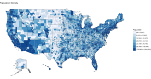
Choropleth – is a thematic map in which areas are shaded or patterned in proportion to the measurement of the statistical variable being displayed on the map, such as population density or per-capita income.

Below is the code for a choropleth, using the package choroplethr and the data set df_pop_county, which is the population of every county in the US.

This is what todays primary objective is;

To learn more about any R command “?”, “??”, or “help(“object”)” Keep in mind, R is case sensitive. If you can only remember part of a command name use apropos().


?str
?df_pop_county
??summary
help(county_choropleth)
apropos("county_")


#Install package called choroplethr, 
#quotes are required, 
#you will get a meaningless error without them
#Only needs to be installed once per machine
install.packages("choroplethr")

The library function will load the installed package to make any functions available for use.


library("choroplethr")

To find out what functions are in a package use help(package=””).

 
help(package="choroplethr")

Many packages come with test or playground datasets, you will use many in classes and many for practice, data(package=””) will list the datasets that ship with a package.


data(package="choroplethr")

For this example we will be using the df_pop_county dataset, this command will load it from the package and you will be able to verify it is available by checking out the Environment Pane in R Studio.


data("df_pop_county")

View(“”) will open a view pane so you can explore the dataset. Similar to clicking on the dataset name in the Environment Pane.


View(df_pop_county)

Part of learning R is learning the features and commands for data exploration, str will provide you with details on the structure of the object it is passed.


str(df_pop_county)

Summary will provide basic statistics about each column/variable in the object that it is passed.


summary(df_pop_county)

If your heart is true, you should get something very similar to the image above after running the following code. county_choropleth is a function that resides in the choroplethr package, it is used to generate a county level US map. The data passed in must be in the format of county number and value, the value will populate the map. WHen the map renders it will be in the plot pane of the RStudio IDE, be sure to select zoom and check out your work.


#?county_choropleth 
county_choropleth(df_pop_county)

There are som additioanl parameters we can pass to the function, use help to find more.


county_choropleth(df_pop_county,
                  title = "Population Density",
                  legend="Population")

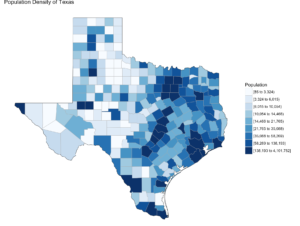
Try changing the number of colors and change the state zoom. If your state is not working read the help to see if you can find out why.


county_choropleth(df_pop_county,
                  title = "Population Density of Texas",
                  legend="Population",
                  num_colors=9,
                  state_zoom="texas")

There is an additional option for county_choropleth, reference_map. If it does not work for you do not fret, as of this blog post it is not working for me either, the last R upgrade whacked it, be ready for this to happen and make sure you have backs and versions, especially before you get up on stage in front 200 people to present.

There you have it! Explore the commands used, look at the other datasets that ship with choroplethr and look at the other functions that ship with choroplethr, it can be tricky to figure out which ones work, be sure to check the help for each function you want to run, no help may mean no longer supported. Remember that these packages are community driven and written, which is good, but sometimes they can be a slightly imperfect.

In the next post i will cover how to upload and create your own dataset and use the choroplethr function with your own data. On a side note, the choropleth falls under a branch of statistics called descriptive statistics which covers visuals used to describe data.