This is a slight diversion into a tool built into R called R Markdown, and Shiny will be coming up in a few days. Why is this important? It gives you a living document you can add text and r scripts to to produce just the output from R. I wrote my Stats grad project using just R Markdown and saved it to a PDF, no Word or open office tools.
Its a mix of HTML and R, so if you know a tiny bit about HTML programing you will be fine, otherwise, use the R Markdown Cheat sheet and Reference Guide which i just annoyingly found out existed…
I am going to give you a full R Markdown document to get you started.
Create a new R Markdown file;

Then Run it by selecting the “Knit” drop down in the middle left of the toolbar and selecting Knit to HTML.
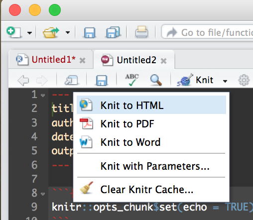
This will create an html document that you can open in a browser, it comes with some default mtcars data just so you can see some output. Try out some R commands and doodle around a bit before starting the code below. This is the file data file we will be using, US-Education.csv It contains just the 2010-2014 educational attainment estimates per count in the US.
In the code books below i will put in each section of the R Markdown and discuss it, each R code block can me moved to r console to be run.
The first section Is the title that will show up on the top of the doc, copy this into the markdown file and run it by itself. I am using an html style tag as i want some of the plots to be two columns across.
You will also see the first R command in an “R” block identified by ““`{r} and terminated with ““`”. Feel free to remove options and change options to see what happens.
Notice below the style tag is wrong, when you copy it out you will need to put the “<" back in from of the style tag. If i format it correctly wordpress takes it as an internal style tag to this post.
---
title: "Educational Attainment by County"

output: html_document
---

style>
  .col2 {
    columns: 2 200px;         /* number of columns and width in pixels*/
    -webkit-columns: 2 200px; /* chrome, safari */
    -moz-columns: 2 200px;    /* firefox */
     line-height: 2em;
     font-size: 10pt;

  }

/style>

```{r setup, include=FALSE}
knitr::opts_chunk$set(echo = FALSE,warning=FALSE)

#require is the fancy version of install package/library
require(choroplethr)

```
This will be the next section in the markup, load a dataframe for each of the four educational attainment categories.
```{r one}

#Load data
 setwd("/data/")
 usa <- read.csv("US-Education.csv",stringsAsFactors=FALSE)

#Seperate data for choropleth
 lessHighSchool <- subset(usa[c("FIPS.Code","Percent.of.adults.with.less.than.a.high.school.diploma..2010.2014")],FIPS.Code >0)

highSchool <- subset(usa[c("FIPS.Code","Percent.of.adults.with.a.high.school.diploma.only..2010.2014")],FIPS.Code >0)

someCollege <- subset(usa[c("FIPS.Code","Percent.of.adults.completing.some.college.or.associate.s.degree..2010.2014")],FIPS.Code >0)

college <- subset(usa[c("FIPS.Code","Percent.of.adults.with.a.bachelor.s.degree.or.higher..2010.2014")],FIPS.Code >0)

#rename columns for Choropleth

 colnames(lessHighSchool)[which(colnames(lessHighSchool) == 'FIPS.Code')] <- 'region'

 colnames(lessHighSchool)[which(colnames(lessHighSchool) == 'Percent.of.adults.with.less.than.a.high.school.diploma..2010.2014')] <- 'value'

#
# or
#
 names(highSchool) <-c("region","value")
 names(someCollege) <-c("region","value")
 names(college) <-c("region","value")


```
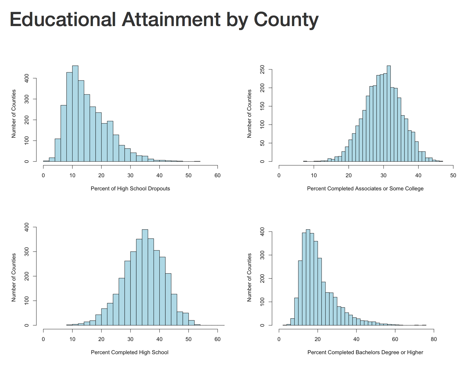
The next section will create four histograms of the college attainment by category. Notice the distribution of the data, normal distribution, right skew, left skew, bimodal? We will discuss them next blog.
Notice for the next section i have the "div" without the left "<", be sure to put those back.
div class="col2">

```{r Histogram 1}
 hist(lessHighSchool$value,xlim=c(0,60),breaks=30, xlab = "Percent of High School Dropouts", ylab="Number of Counties",main="",col="lightblue")


 hist(highSchool$value,xlim=c(0,60),breaks=30, xlab = "Percent Completed High School ", ylab="Number of Counties",main="",col="lightblue")

```


```{r Histogram 2}

 hist(someCollege$value,xlim=c(0,50),breaks=30, xlab = "Percent Completed Associates or Some College ", ylab="Number of Counties",main="",col="lightblue")

 hist(college$value,xlim=c(0,90),breaks=30, xlab = "Percent Completed Bachelors Degree or Higher ", ylab="Number of Counties",main="",col="lightblue")


```

/div>
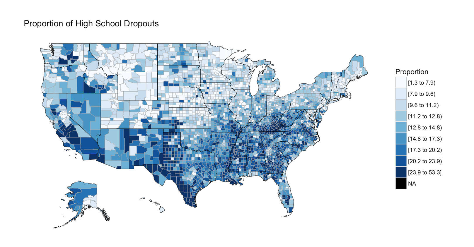
The next section is the choropleth, for the high school dropouts, notice the R chunk parameters to size the plot area.
```{r two, fig.width=9, fig.height=5, fig.align='right'}


 county_choropleth(lessHighSchool,

                   title = "Proportion of High School Dropouts",
                   legend="Proportion",
                   num_colors=9)

```
There are three more choropleths that you will have to do on your own! you have the data, and the syntax. If you have trouble with this, the red file i used is here Education.rmd
In the end, you should have a histogram looking like this;
And if you make it to the first choropleth, Percentage that did not complete high school;