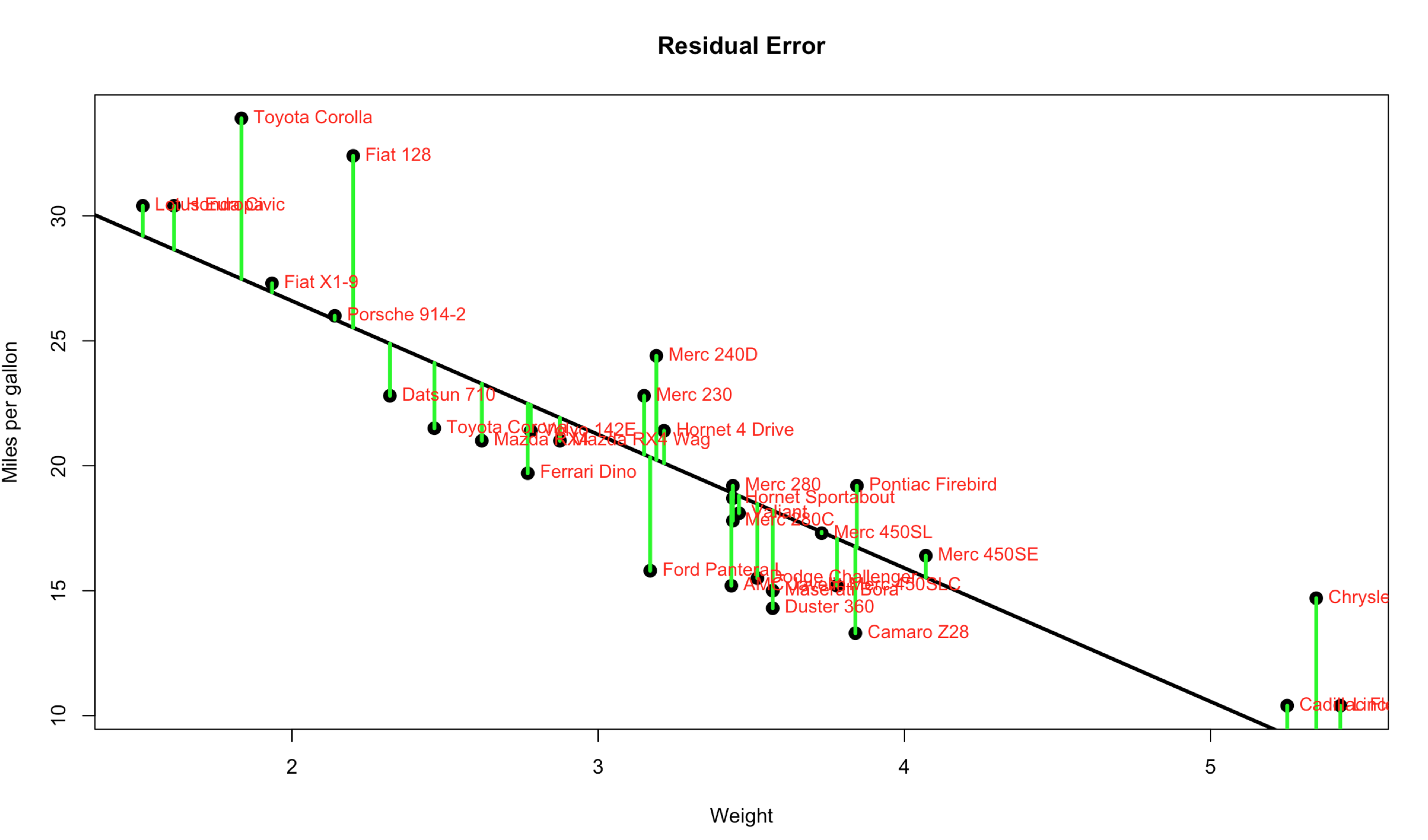
All the numbers, so many numbers, do we really need all of them…? If you want to make a an informed decision yes, you do. On the bright side they are not very hard to interpret, almost all of the numbers are related to just one number… The Error, more specifically the Residual Error. I’m going to blow your hair back again, its not an error, its nothing like and error, it should have never been called an error, its a difference. It is the difference between the line we ran through the middle of the scatter plot and the data points. Each point has a difference between the line and where the dot falls. Take a look at the visual below, the green line represents the distance between the line and the actual data point, thats our residual error. Its not hard to see that the larger the distance between the line and the data points the worse our model will perform. Not to mention the closer the data is to the the better.

Code for this is below if you want to adapt your own, I am 99% sure i grabbed this out of the ISLR at some point in the last two years, they show a sample on page 62, for lack of exact page and section of code just get your own copy, i consider ISLR a necessary resource.

plot(mtcars$mpg~mtcars$wt,
     cex=1.5, 
     pch=16,
     xlab="Weight",  #X axis label
     ylab="Miles per gallon",
     main = "Residual Error") #Y axis label)
abline(lm(mtcars$mpg ~ mtcars$wt),
       lwd=3, 
       col="black")
text(mtcars$wt, mtcars$mpg, row.names(mtcars), cex=0.9, pos=4, col="red")

mtcars.1 <- lm(mtcars$mpg ~ mtcars$wt)

summary(mtcars.1)
#Add some lines between the line and the actual to demonstrate the error
yhat <- predict(mtcars.1 , tfr = mtcars$wt)
join <- function(i) 
  lines(c(mtcars$wt[i],mtcars$wt[i]),c(mtcars$mpg[i],yhat[i]),col="green",lwd=3) 
sapply(1:32,join)

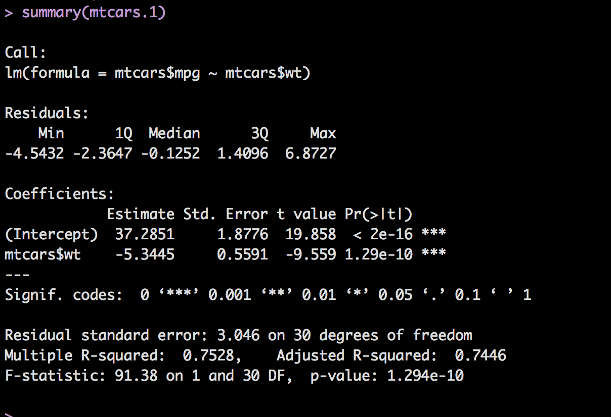
Going back to our output from the summary of our model we can start with the first section, Residuals.

One thing i want to point out in my scripts is how i qualify the variables when passed into lm(). The correct way, "lm(mpg ~ wt, data=mtcars)" the wrong way; "lm(mtcars$mpg ~ mtcars$wt)". The wrong way will work, but will bite you in the butt when you get to prediction. You will see both in my posts, i get lazy and just type it out without paying much attention, but, its not a good habit to get into. So do as i say and not as id do and be sure to add data= when qualifying your dataset. I will try and do better in the future.

You can get a vague idea of the distribution of the residual errors by looking at a histogram or a plot of them, or plot the entire model with one command. If you want to know where that comes from just run the code below. Now another frustration, depending on who is teaching everyone has a different opinion about what is useful. I have included what to look for in each, regardless of opinions.

# Not much, make sure numbers are not hugely far away from zero, 
# be aware fo scale. 
summary(mtcars.1$residuals)

# Scattered all about the plot is the generic explanation.
# If the data is clustered in one area the model will lean towards satisfying that data 
# but stink at predicting other data. 

plot(mtcars.1$residuals)

# Generally looking for normal distrbution 
hist(mtcars.1$residuals)

# hit enter in the console after each plot, 
# or set par(mfrow=c(2,2)) to see them all together

par(mfrow=c(2,2))
plot(mtcars.1)

# if you want to have some fun figure out the mean of the residuals, 
# since we have scipen=999 you will never get exact zero, but its zero.  
# Mean of the residuals will always be zero. 

mean(mtcars.1$residuals)

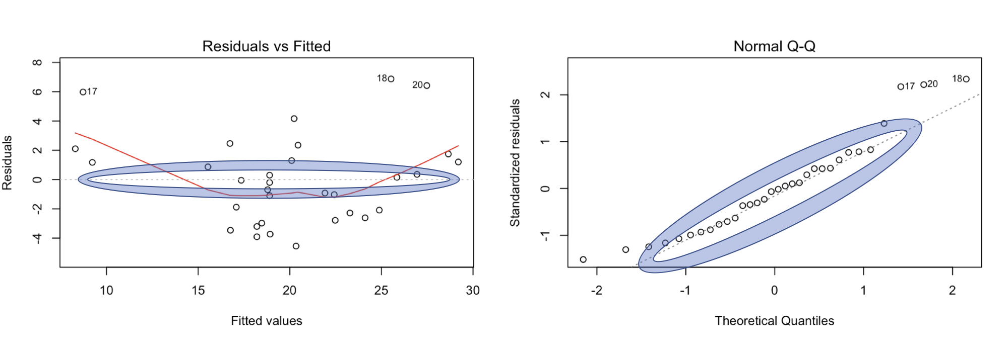
Form the plot(mtcars.1), the first two graphs are what to focus on, this is very subjective, but once you have done this with a few datasets it will make sense. You want the residual vs fitted to be as close to zero as possible, in this case the data is all over the place, the line is using something called smoothing to give you an idea where the data is concentrated or leaning, you will notice some of the points have numbers, those are outliers, which usually means more than two standard deviations away from the mean of the residual errors.

The Normal Q-Q should have all the points on or hugging the line, but ours looks a bit jagged and the far left and far right are way off the line indicating we will have trouble predicting low mpg cars, and very high mpg cars. In other words, based on the Residual Errors, we may not have the best data set or weight is a less than stellar explanatory variable, though clearly has some value.

Moving along with the output from summary(mtcars.1), with one change, if you run options(scipen=999) R will drop the scientific notation and show you the entire number, be careful with this as a computer has no concept of zero so some things you expect to be zero may now become an extremely small number.

The Coefficient Estimate was discussed in the last post, essentially the intercept and slope, next is the standard error, in short it is the average expected error for a single prediction. ISLR page 65 discusses this, the average the prediction differs from the actual, the lower the better.

T-Value is the Estimate divided by the Standard error, the farther from 1 the better. You can imagine based on the description of Standard error that if the estimate is 37 and the error is 37 our model is horrible, and t-value would be 1.

The last column is "Pr(>|t|)" (or p-value) here is what that means in english; The Probability of the absolute value of T occurring randomly in the world. In other words, is this variable Weight useful in predicting mpg or is it nonsense. A value of <.05 is typically considered a good predictor of usefulness of the variable, but that too is subjective. For multiple regression all of these must be taken into consideration. Signif. codes: is your cheat sheet, R tries to help you by placing 1,2 or 3 stars next to a coefficient so you can easily tell if it is useful or not, always look at the actual p-value.

Next is the "Residual standard error: 3.046 on 30 degrees of freedom" or the RSE, RSE is the Sum of Squared Errors/Degrees of freedom. Wait, what? RSE is a quotient i have never heard of with a thing divided by another thing i have never heard of. So, remember when i said the software will do it for you, this could be one of those moments... So what i am going to do instead is create a post with just these numbers and where they all come from, and then provide you an excel spreadsheet so if you want to plug in all of your own values and see what happens, you can.

More tomorrow....