I think it’s difficult for a professor or teacher to know at exactly what point should linear regression be taught in a curriculum, it seems like it turns up everywhere calculus, algebra stats, modeling. It should be in all of them, but then the next question is do you need to know algebra, matrix algebra and linear algebra before knowing how to do a linear regression? I don’t know to be honest. Having worked with SQL for most of my adult life I have had to know and use all three and did not pay much attention to it or realize until I started formally beefing up my academics.
Regardless, the one thing I have heard from a few stats instructors is “don’t worry about how its done or how it works, the software will take care of it for you”, to be fair, these were not stats professors at the local beauty college, these were ivy league educated (I checked) professors and teachers saying this. Which, my problem is if I don’t know how it works I will probably not truly understand it, ever. Depending on what you are doing a trivial knowledge may be sufficient, but what if it’s not? If I am in an interview can I use the words “the software will do it for me” as the answer to a hard question?
What?
In the next few posts, I will do my best to define Linear Regression in R using lm. Your first question should be when do I use lm or linear regression to solve a problem. In short, you have a quantitative explanatory variable and a quantitative predictor. Yup, already lost you huh? Here is the deal, I am going to use the mtcars (motor trend cars 1974) dataset because everyone uses it and its super simple to understand. Let’s start with a hypothesis, or an idea i want to test; if a car increases in weight does the gas mileage go up, down or stay the same? Stays the same would be the null hypothesis if you are keeping track, does not stay the same would be the alternative hypothesis. But, if you are not ready for hypo testing just move along don’t sweat it and keep going.
One item to clear up is the difference in Simple Linear Regression and Multiple Linear Regression; Simple has one explanatory variable, Multiple has more than one. I know right? Your hair is blown back by that piece of complex knowledge.
How?
To start with we need some data and luckily have that.
I will provide an R script at the very end of this lm series, I will include code bits I cover here, data exploration is an important part of the discovery process, be sure to look at all of the variables, not just weight.
A good starting point for any exploration of data is quite simply looking at the data, perform some basic descriptive statistics on the data and make sure you have some understanding of what it is.
data(mtcars)
head(mtcars)
View(mtcars)

summary(mtcars)

summary(mtcars$wt)
summary(mtcars$mpg)

str(mtcars)
If you are outside of the US the first thing you may want to do is convert mpg to liters per 100 kilometers so this data set makes more sense to you.
So if you must;
1 US gallon is equal to 3.785 liters
1 Mile is equal to 1.609 Kilometers
Liters per 100 kilometer = (100 * 3.785) / (1.609 * MPG)
# If you absolutely must convert, here you go
mtcars$lp100k <- (100 * 3.785) / (1.609 * mtcars$mpg)
plot(mtcars$mpg ~ mtcars$wt,
     main = "MTCars Weight");
Continue to explore a bit to see if there appears to be a relationship between x and y, or weight and miles per gallon or liters per 100k. Specifically, we can start with an XY scatter chart to see if we can find anything interesting.
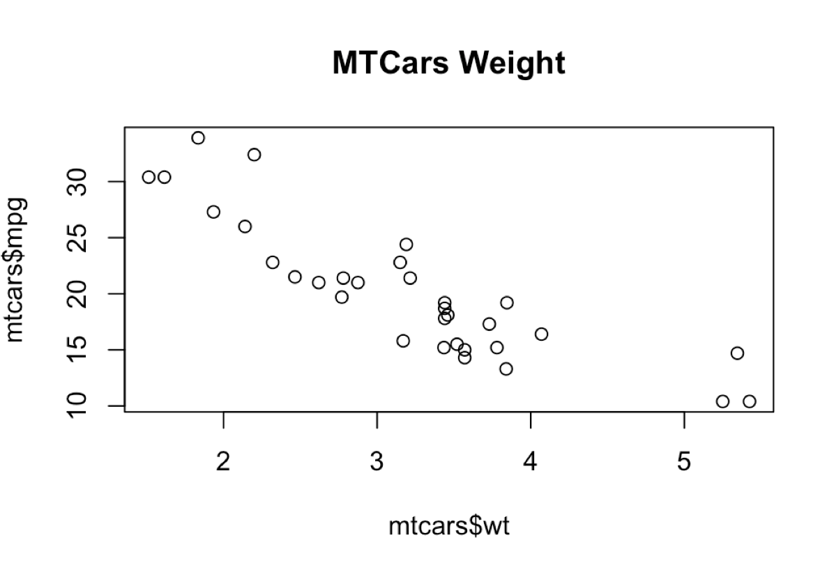
With very little we can get a scatter plot and just looking we can see there appears that as weight decreases, (weight of 2 = 2000 pounds) miles per gallon increase. Though jagged and scattered, it does look like something is here.
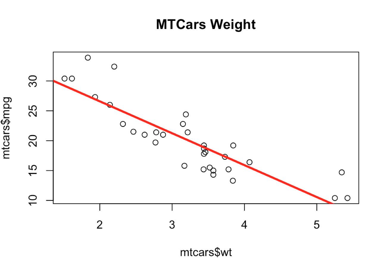
Now we can use a linear regression line to see what it will look like by adding the abline command and passing the results of an lm to it. I will explain how that line magic happens later on.
abline(lm(mpg ~ wt,data=mtcars),
       lwd=3,
       col="red")
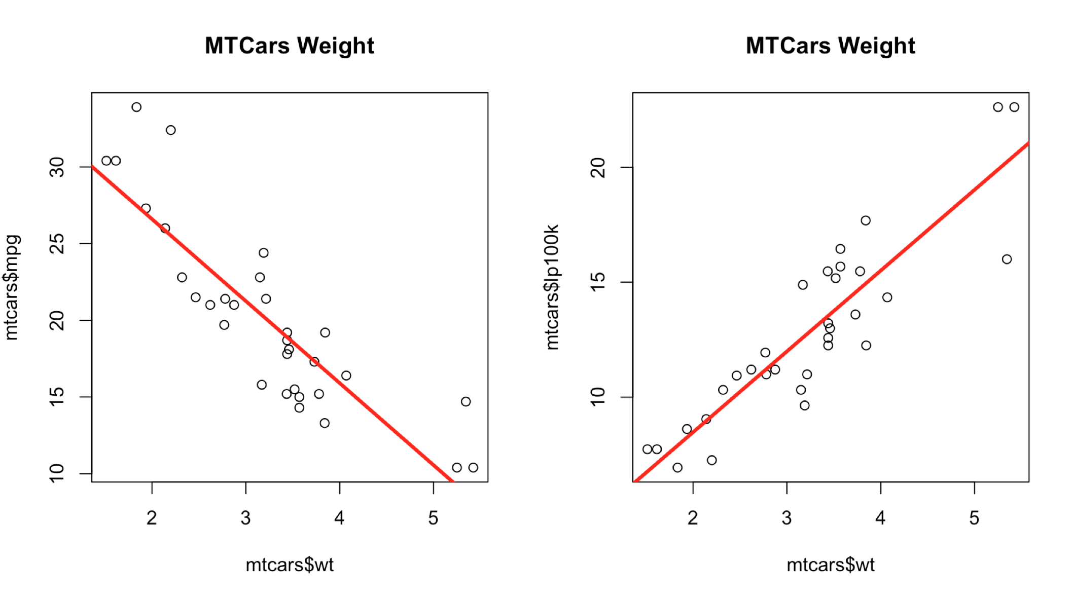
For fun lets add the new variable for our European and Canadian friends. For this lets plot the two side by side using par(mfrow=c(rows,columns)).
par(mfrow=c(1,2))

plot(mtcars$mpg ~ mtcars$wt,
     main = "MTCars Weight");
abline(lm(mpg ~ mtcars,data=mtcars),
       lwd=3,
       col="red")


plot(mtcars$lp100k ~ mtcars$wt,
     main = "MTCars Weight");
abline(lm(lp100k ~ wt,data=mtcars),
       lwd=3,
       col="red")
Without thinking your first response is converting to liters gives me better gas mileage... NOPE... This is actually a prefect example of what happens when you convert a unit of measure to another unit of measure. We went form measuring the miles we travel using one gallon of fuel vs how many liters it takes to travel 100 kilometers, its completely reversed and at a different scale. The line and the dots are the same in both charts, but sort of reversed from each other. If you have some doubt you can add labels to the plot by adding "text(mtcars$wt, mtcars$lp100k, row.names(mtcars), cex=0.9, pos=4, col="red")" after the abline command. Be sure to change the y axis for mpg if you go back and forth.
But for now, our basic question was is there a relationship between the weight and miles per gallon, from a cursory look at the data, I would say yes, and there does appear to be a somewhat linear relationship.
The next step in our process is to see if we can fit a model to the data, that means can we take the data we have and use it to predict the miles per gallon of a vehicle if we know the weight with some level of certainty?
Lets create a model... The following command will create a linear regression model using mpg as the predictor and wt(weight) as the explanatory variable. You can just as easily replace mpg with lp100k if you prefer.
mtcars.1 <- lm(mtcars$mpg ~ mtcars$wt)
If you did it correctly, there is nothing in the console and a new list in the global environment called mtcars.1. To get some useful meat out of this thing we just created we use summary().
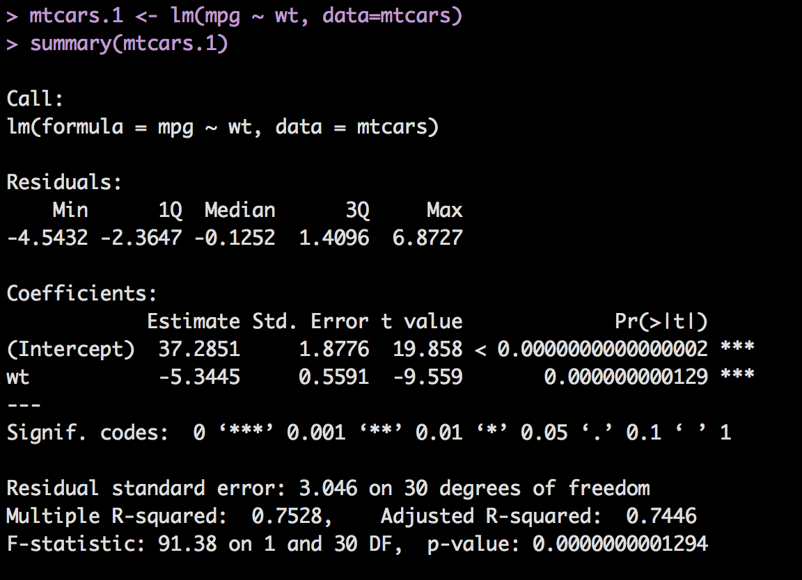
What is all of that mess and does any of it actually matter? Yes. It matters, we will go through all of it. Two things i want to point out in this post is R-Squared and Coefficients.
R-Squared
First the R-Squared, as general rule of thumb, though there are dozens of exceptions to this rule, the closer to 1.0 the R-Squared is the better the model is at predicting something. You can only use the R-Squared when you have one explanatory variable, we have wt(weight) to predict mpg and nothing else, otherwise use adjusted r-squared, more on that later. The simplest definition of R-Squared; 75.8% of the variability in the data is accounted for by the model. Another way of saying it, R square is a way of measuring the relationship between x and y, or in this case mpg and wt. 1 is a perfect fit, if it is close to zero then x and y must have nothing to do with each other.
Coefficients
What does all this numeric jibber jabber mean? Focusing on just Estimate and the (intercept) and mtcars$wt. You have actually seen this already but were unaware of it. In the scatter plot where we had the line through the plot we ran lm() inside the abline function and a line magically appeared? So, what magic was that? if you run lm() and do not save it to a data frame it will return and intercept coordinate and a slope coordinate. In this case 37.2851 as the intercept which means that the line will cross zero on the y axis at 37.2851 mpg and have a slope of -5.3445. If we take the original scatter plot and feed in just the numbers you will see the same line.
plot(mpg~wt,data=mtcars,
     cex=1,
     pch=16);
abline(37.2851, -5.3445,
       lwd=3,
       col="red")
You can run it, i have already seen it. But, what does this really mean? Recall that wt is in thousands, 1.0 = 1,000 pounds, 2 = 2,000 pounds, 3.440 = 3,440 pounds etc. For the dataset they were all divided by 1000. What the scatter plot and lm tell us is that for every 1 unit (1000 pound) increase in weight the mpg will decrease by 5.3445 miles per gallon on average based on the data we have provided.
Thats is all for today. Play with the scatter plot and creating more models and looking at the coefficients. Try replacing wt with hp(horse power), qsec(quarter mile time), etc, even try replacing y with something else.
To learn more about the dataset "?mtcars"