Monthly Archives: January 2017

Visualization, Histogram

Published / by shep2010

So, last blog we covered a tiny bit of vocabulary, hopefully it was not too painful, today we will cover a little bit more about visualizations. You have noticed by now that R behaves very much like a scripting language which having been a T-SQL guy seemed familiar to me. And you have noticed that it behaves like a programing language in that I can install a package, and invoke function or data set stored in that package, very much like a dll, though no compiling is required. It’s clear that it is very flexible as a language, which you will learn is its strength and its downfall. If you decide to start designing your own R packages, you can write them as terribly as you want, though i would rather you didn’t.

If you want to find out what datasets are available run “data()”, and as we covered in a prior blog, data(package=) will give you the datasets for a specific package. This will provide you nice list of datasets to doodle with, as you learn something new explore the datasets to see what you can apply your new-found knowledge to.

First lets check out the histogram. If you have worked with SQL you know what a histogram is, and it is marginally similar to a statistics visual histogram. We are going to look at a real one. The basic definition is that it is a graphical representation of the distribution of numerical data.

When to use it? When you want to know the distribution of a single column or variable.

“Hist” ships with base R, which means no package required. We will go through a few Histograms from different packages.

You have become familiar with this by now, “data()” will load the mtcars dataset for use, “View” will open a new pane so you can review it, and help() will provide some information on the columns/variables in the dataset. Fun fact, if you run “view” (lowercase v) it will display the contents to the console, not a new pane. “?hist” will open the help for the hist command.


data(mtcars)
View(mtcars)
help(mtcars)

?hist

Did you notice we did not load a package? mtcars ships with base R, run “data()” to see all the base datasets.

Hist takes at a single quantitative variable, this can be passed by creating a vector or referencing just the dataframe variable you are interested in.

Try each of these out one at a time.


#When you see the following code, this is copying the contents 
#of one variable into a vector, it is not necessary for what 
#we are doing but it is an option. Once copied just pass it in to the function. 

cylinders <- mtcars$cyl
hist(cylinders)

#Otherwise, invoke the function and pass just the variable you are interested in.

hist(mtcars$cyl)
hist(mtcars$cyl, breaks=3)
hist(mtcars$disp)
hist(mtcars$wt)
hist(mtcars$carb)

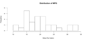
As you get wiser you can start adding more options to clean up the histogram so its starts to look a little more appealing, inherently histograms are not visually appealing but they are a good for data discovery and exploration. Without much thought you can see that more vehicles get 15mpg.


hist(mtcars$mpg, breaks = 15)

hist(mtcars$mpg, breaks = 15,
    xlim = c(9,37),
    ylim = c(0,8),
    main = "Distribution of MPG",
    xlab = "Miles Per Gallon")

Lets kick it up a notch, now we are going to use the histogram function from the Mosaic package. The commands below should be looking familiar by now.


install.packages("mosaic")
library(mosaic)

help(mosaic)

Notice there is more than one way to pass in our dataset. Since histogram needs a vector, a dataset with one column, any method you want to use to create that on the fly will probably work.


#try out a set of numbers
histogram(c(1,2,2,3,3,3,4,4,4,4))

#from the mtcars dataset let look at mpg and a few others and try out some options
histogram(mtcars$mpg)

#Can you see the difference in these?  which is the default? 
histogram(~mpg, data=mtcars)
histogram(~mpg, data=mtcars, type="percent")
histogram(~mpg, data=mtcars, type="count")
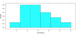
histogram(~mpg, data=mtcars, type="density")

Not very dazzling, but it is the density of the data. This is from "histogram(mtcars$mpg)"

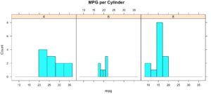
Well, this is all sort of interesting, but quite frankly it is still just showing a data density distribution. Is there away to add a second dimension to the visual without creating three histograms manually? Well, sort of, divide the data up by a category.

While less pretty with this particular dataset, you can see that it divided the histograms up by cylinders using the "|". You will also notice that i passed in "cyl" as a factor, this means treat it as a qualitative value, without the "as.factor" the number of cylinders in the label will not display, and that does not help with readability. Remove the as.factor to see what happens. Create your own using mtcars.wt and hp, do any patterns emerge?


histogram(~mpg | as.factor(cyl), 
          main = "MPG per Cylinder",
          data=mtcars, 
          center=TRUE,
          type="count", 
          n=4, 
          layout = c(3,1))

Well that was fun, remember when i said lets kick it up a notch? Here we go again. My favorite, and probably the most popular R visualization packages is ggplot or more recently, GGPLOT2


install.packages("ggplot2")
library(ggplot2)

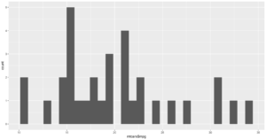
qplot(mtcars$mpg, geom="histogram") 

WOW, the world suddenly looks very different, just the default histogram look as if we have entered the world of grown up visualizations.

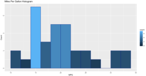
Ggplot has great flexibility. Check out help and search the web to see what you can come up with on your own. The package worth of an academic paper, or if you want to dazzle your boss.


ggplot(data=mtcars, aes(mtcars$mpg),) + 
  geom_histogram(breaks=seq(10, 35, by =2),
    col="darkblue",
    aes(fill=..count..))+
    labs(title="Miles Per Gallon Histogram") +
    labs(x="MPG", y="Count")

Todays Commands

Base R
data()
View()
help()
hist()
install.packages()
library()

Mosaic Package
histogram

Ggplot2 Package
qplot()
ggplot()
geom_histogram()

Shep
Stats stuff 1 In the beginning

Published / by shep2010

There is no escaping it, you are going to have to know some stat stuff. Every now and then I will through in a blog post to cover some of this, its good for me to attempt to brain dump it, and its good for you to try and assimilate it. Nothing is going to make sense without it. It only hurts a little bit and I am going to try and give as many samples as possible and break down each concept as much as I possibly can. In the end you will be grateful for software, but stats came from long hand math calculations and have formulas that look like they could single handledly put a rocket in space.

If you are a RDBMS gal or guy some of the definitions will seem wonky, and if you are talking to an academic this will be the first communication breakdown, hopefully this will help.

Lets get some definitions out of the way, these are critical, it does not mean you need to question the lingo you use on a daily basis, but if you hear it from you statisticians or DS folks, make sure you are on the same page.

Population – A population is ALL THE DATA. As a data guy I lived in a world where if we were trying to make a decision we used all the data, this is why we had SQL performance problems, our customers sucked at statistics and did not know there was a way to sample a data set. That being said, i also would not like to check my bank account balance based on a sample. So, when you see a population referenced that means the entire data, all of it. If I am using a population of the United States, that means I am using all 330 million or so people in the US for my research. In Statistics, it is denoted as an uppercase N.

Census – A census is a study of EVERYTHING in a given population. Most countries have a census. One of the more popular results of the census is the American Community Survey, it frequently provides great statistical training and research material.

Sample – A sample is as it sounds, it’s a sample of a population, hence not all the data. There are sub-classes of samples we will get into later. But for now know that a sample is a portion of a population. In Statistics, it is denoted as an lowercase n.

Parameter – A parameter is a numerical quantity that tells us something about the population, such as quantity of a specific ethnicity, number high school graduates, proportion of singles. Do not confuse this with a numeric quantity of sample, that is called a statistic. Ah ha!

Variable – A variable in statistics is what most SQL Folks, me included call a column, there is a very long definition, they contain anything that describe a characterization, qualitative and quantitative.

Case – A case in statistics is a single row of data. You can imagine that if you have a patient, all of the columns(variables) will make up the data for that patient, hence it is called a case. So, if you hear this outside of academia see if they are discussing a row, or something else entirely. Usually, this terminology references something sciencey, less so outside of medical research or scientific fields. I have never heard a row of banking data referred to as a case.

Data – Plural for of data. Some get bent out of shape over the use of this, I find them more annoying than the usage, I mean its not like I am using there their they’re incorrectly.

Datum – Singular form of data.

Qualitative Data – In many respects this is an easy one, if its not Quantitative its probably Qualitative, another more familiar name for it is categorical or, a category. Categorical data is defined as which? Which color, which model of, which dog breed, which grade are you in.

If you recall, looking at the dataset we used for the Florida education choropleth you will recall that there was a variable called ruralurbancontinuum , though it was a number it was used as a categorical value. The values of this field are 1-9 and related to a category of population density used US wide. In this case no math could be done gainst the value even though it is a number, the Census could just have easily used A-I instead of 1-9.

Quantitative Data – This one is pretty easy if you remember that you can do math on a quantitative variable. Its is always a number. It can be my height, my weight, my pulse rate, the money in my checking account, my shoe size. If I have population or sample of these items I can average them, get a standard deviation etc. The word quantitative has a root of quantity, that should help you remember it.

To go a little bit deeper into the rabbit whole there are two types of Quantitative data, I know, I’m sorry… Hopefully looking at the root word of each will help.

Quantitative Discreet – Counting data. They ask How Many?

How many people on a bus?
-There are 20 people on the bus, not 19.5 or 20.5.

How many cars in my driveway?
-There are 2 cars in my driveway and one in the yard, though most of that on is missing it is still one car.

How many books do you own?
-I own 100 books, not 99.5, though an argument could be made for owning half a book, it is still one registered ISBN even if you do not have all of the book.

How many emails did you get to day?
-I received 50 emails today.

Quantitative Continuous – Measuring data, this asks How Much?

What is your height?
What is your weight?
What is the weight of a vehicle?
What ii the MPG of a vehicle?

The following sources help with statistics, FOR FREE

Khan academy of course, as well as;

Introductory Statistic, OpenStax

OpenIntro Statistics

Australian Bureau of Statistics, Go figure, their definitions are too the point