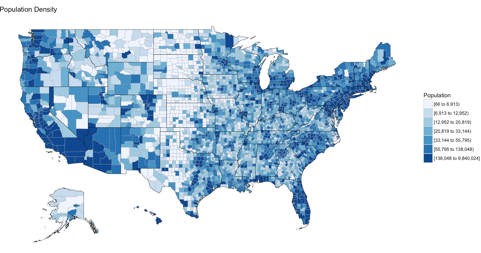
In the last blog you were able to get a dataset with county and population data to display on a US map and zoom in on a state, and maybe even a county if you went exploring. In this demo we will be using the same choroplethr package but this time we will be using external data. Specifically, we will focus on one state, and check out the education level per county for one state.
The data is hosted by the USDA Economic Research Division, under Data Products / County-level Data Sets. What will be demonstrated is the proportion of the population who have completed college, the datasets “completed some college”, “completed high school”, and “did not complete high school” are also available on the USDA site.
For this effort, You can grab the data off my GitHub site or the data is at the bottom of this blog post, copy it out into a plain text file. Make sure you change the name of the file in the script below, or make sure the file you create is “Edu_CollegeDegree-FL.csv”.
Generally speaking when you start working with GIS data of any sort you enter a whole new world of acronyms and in many cases mathematics to deal with the craziness. The package we are using eliminates almost all of this for quick and dirty graphics via the choroplethr package. The county choropleth takes two values, the first is the region which must be the FIPS code for that county. If you happen to be working with states, then the FIPS state code must be used for region. To make it somewhat easier, the first two digits of the county FIPS code is the state code, the remainder is the county code for the data we will be working with.
So let’s get to it;
Install and load the choroplethr package
install.packages("choroplethr")
library(choroplethr)
Use the setwd() to set the local working directory, getwd() will display what the current R working directory.
setwd("/Users/Data")
getwd()
Read.csv will read in a comma delimited file. “<-“ is the assignment operator, much like using the “=”. The “=” can be used as well. Which to assignment operator to use is a bit if a religious argument in the R community, i will stay out of it.
# read a csv file from my working directory
edu.CollegeDegree <- read.csv("Edu_CollegeDegree-FL.csv")
View() will open a new tab and display the contents of the data frame.
View(edu.CollegeDegree)
str() will display the structure of the data frame, essentially what are the data types of the data frame
str(edu.CollegeDegree)
Looking at the structure of the dataframe we can see that the counties imported as Factors, for this task it will not matter as i will not need the county names, but in the future it may become a problem. To nip this we will reimport using stringsAsFactors option of read.csv we will get into factors later, but for now we don't need them.
edu.CollegeDegree <- read.csv("Edu_CollegeDegree-FL.csv",stringsAsFactors=FALSE)

#Recheck our structure
str(edu.CollegeDegree)
Now the region/county name is a character however, the there is actually more data in the file than we need. While we only have 68 counties, we have more columns/variables than we need. The only year i am interested in is the CollegeDegree2010.2014 so there are several ways to remove the unwanted columns.
The following is actually using index to include only columns 1,2,3,8 much like using column numbers in SQL vs the actual column name, this can bite you in the butt if the order or number of columns change though not required for this import, header=True never hurts. You only need to run one of the following commands below, but you can see two ways to reference columns.
edu.CollegeDegree <- read.csv("Edu_CollegeDegree-FL.csv", header=TRUE,stringsAsFactors=FALSE)[c(1,2,3,8)]

# or Use the colun names

edu.CollegeDegree <- read.csv("Edu_CollegeDegree-FL.csv", header=TRUE,stringsAsFactors=FALSE)[c("FIPS","region","X2013RuralUrbanCode","CollegeDegree2010.2014")]

#Lets check str again
str(edu.CollegeDegree)
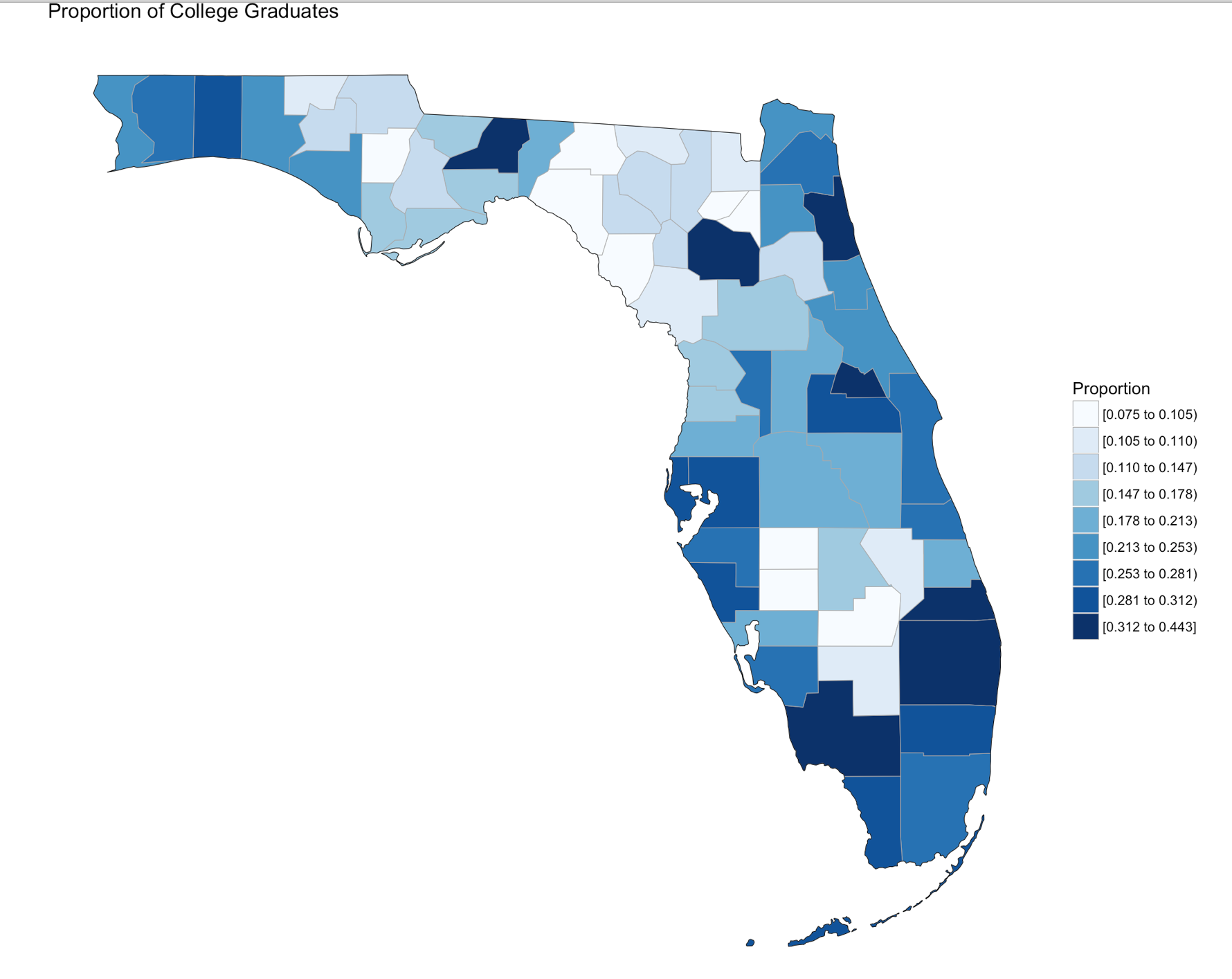
Using summary() we can start reviewing the data from statistical perspective. The CollegeDegree2010.2014 variable, we can see the county with the lowest proportion of college graduates is .075, or 7.5% of the population of that county the max value is 44.3%. The average across all counties is 20.32% that have completed college.
summary(edu.CollegeDegree)
Looking at the data we can see that we have a FIPS code, and the only other column we are interested in for mapping is CollegeDegree2010.2014, so lets create a dataframe with just what we need.
View(edu.CollegeDegree)

# the follwoing will create a datafram with just the FIPS and percentage of college grads
flCollege <- edu.CollegeDegree[c(1,4)]

# Alternatively, you can use the column names vs. the positions. Probably smarter ;-)
flCollege <- edu.CollegeDegree[c("FIPS","CollegeDegree2010.2014")]

# the following will create a dataframe with just the FIPS and percentage of college grads

flCollege
But, from reading the help file on county_choropleth, it requires that only two variables(columns) be passed in, region, and value. Region must be a FIPS code so, we need to rename the columns using colnames().
colnames(flCollege)[which(colnames(flCollege) == 'FIPS')] <- 'region'
colnames(flCollege)[which(colnames(flCollege) == 'CollegeDegree2010.2014')] <- 'value'
So, lets map it!
Since we are only using Florida, set the state_zoom, it will work without the zoom but you will get many warnings. You will also notice a warning that 12000 is not mappable. Looking at the data you will see that 12000 is the entire state of Florida.
county_choropleth(flCollege,
                  title = "Proportion of College Graduates ",
                  legend="Proportion",
                  num_colors=9,
                  state_zoom="florida")
For your next task, go find a different state and a different data set from the USDA or anywhere else for that matter and create your own map. Beware of the "value", that must be an integer, sometimes these get imported as character if there is a comma in the number. This may be a good opportunity for you to learn about gsub and as.numeric, it would look something like the following command. Florida is the dataframe, and MedianIncome is the column.
florida$MedianIncome <- as.numeric(gsub(",", "",florida$MedianIncome))
USDA Economic Research Division Sample Data
FIPS,region,2013RuralUrbanCode,CollegeDegree1970,CollegeDegree1980,CollegeDegree1990,CollegeDegree2000,CollegeDegree2010-2014
12001,"Alachua, FL",2,0.231,0.294,0.346,0.387,0.408
12003,"Baker, FL",1,0.036,0.057,0.057,0.082,0.109
12005,"Bay, FL",3,0.092,0.132,0.157,0.177,0.216
12007,"Bradford, FL",6,0.045,0.076,0.081,0.084,0.104
12009,"Brevard, FL",2,0.151,0.171,0.204,0.236,0.267
12011,"Broward, FL",1,0.097,0.151,0.188,0.245,0.302
12013,"Calhoun, FL",6,0.06,0.069,0.082,0.077,0.092
12015,"Charlotte, FL",3,0.088,0.128,0.134,0.176,0.209
12017,"Citrus, FL",3,0.06,0.071,0.104,0.132,0.168
12019,"Clay, FL",1,0.098,0.168,0.179,0.201,0.236
12021,"Collier, FL",2,0.155,0.185,0.223,0.279,0.323
12023,"Columbia, FL",4,0.083,0.093,0.11,0.109,0.141
12027,"DeSoto, FL",6,0.048,0.082,0.076,0.084,0.099
12029,"Dixie, FL",6,0.056,0.049,0.062,0.068,0.075
12031,"Duval, FL",1,0.089,0.14,0.184,0.219,0.265
12033,"Escambia, FL",2,0.092,0.141,0.182,0.21,0.239
12035,"Flagler, FL",2,0.047,0.137,0.173,0.212,0.234
12000,Florida,0,0.103,0.149,0.183,0.223,0.268
12037,"Franklin, FL",6,0.046,0.09,0.124,0.124,0.16
12039,"Gadsden, FL",2,0.046,0.086,0.112,0.129,0.163
12041,"Gilchrist, FL",2,0.027,0.071,0.074,0.094,0.11
12043,"Glades, FL",6,0.031,0.078,0.071,0.098,0.103
12045,"Gulf, FL",3,0.057,0.068,0.092,0.101,0.147
12047,"Hamilton, FL",6,0.055,0.059,0.07,0.073,0.108
12049,"Hardee, FL",6,0.045,0.074,0.086,0.084,0.1
12051,"Hendry, FL",4,0.076,0.076,0.1,0.082,0.106
12053,"Hernando, FL",1,0.061,0.086,0.097,0.127,0.157
12055,"Highlands, FL",3,0.081,0.097,0.109,0.136,0.159
12057,"Hillsborough, FL",1,0.086,0.145,0.202,0.251,0.298
12059,"Holmes, FL",6,0.034,0.06,0.074,0.088,0.109
12061,"Indian River, FL",3,0.107,0.155,0.191,0.231,0.267
12063,"Jackson, FL",6,0.064,0.081,0.109,0.128,0.142
12065,"Jefferson, FL",2,0.061,0.113,0.147,0.169,0.178
12067,"Lafayette, FL",9,0.048,0.085,0.052,0.072,0.116
12069,"Lake, FL",1,0.091,0.126,0.127,0.166,0.21
12071,"Lee, FL",2,0.099,0.133,0.164,0.211,0.253
12073,"Leon, FL",2,0.241,0.32,0.371,0.417,0.443
12075,"Levy, FL",6,0.051,0.078,0.083,0.106,0.105
12077,"Liberty, FL",8,0.058,0.08,0.073,0.074,0.131
12079,"Madison, FL",6,0.07,0.083,0.097,0.102,0.104
12081,"Manatee, FL",2,0.096,0.124,0.155,0.208,0.275
12083,"Marion, FL",2,0.074,0.096,0.115,0.137,0.172
12085,"Martin, FL",2,0.079,0.16,0.203,0.263,0.312
12086,"Miami-Dade, FL",1,0.108,0.168,0.188,0.217,0.264
12087,"Monroe, FL",4,0.091,0.159,0.203,0.255,0.297
12089,"Nassau, FL",1,0.049,0.091,0.125,0.189,0.23
12091,"Okaloosa, FL",3,0.132,0.166,0.21,0.242,0.281
12093,"Okeechobee, FL",4,0.047,0.057,0.098,0.089,0.107
12095,"Orange, FL",1,0.116,0.157,0.212,0.261,0.306
12097,"Osceola, FL",1,0.067,0.092,0.112,0.157,0.178
12099,"Palm Beach, FL",1,0.119,0.171,0.221,0.277,0.328
12101,"Pasco, FL",1,0.049,0.068,0.091,0.131,0.211
12103,"Pinellas, FL",1,0.1,0.146,0.185,0.229,0.283
12105,"Polk, FL",2,0.088,0.114,0.129,0.149,0.186
12107,"Putnam, FL",4,0.062,0.081,0.083,0.094,0.116
12113,"Santa Rosa, FL",2,0.098,0.144,0.186,0.229,0.265
12115,"Sarasota, FL",2,0.142,0.177,0.219,0.274,0.311
12117,"Seminole, FL",1,0.094,0.195,0.263,0.31,0.35
12109,"St. Johns, FL",1,0.085,0.144,0.236,0.331,0.414
12111,"St. Lucie, FL",2,0.081,0.109,0.131,0.151,0.19
12119,"Sumter, FL",3,0.047,0.07,0.078,0.122,0.264
12121,"Suwannee, FL",6,0.056,0.065,0.082,0.105,0.119
12123,"Taylor, FL",6,0.064,0.086,0.098,0.089,0.1
12125,"Union, FL",6,0.033,0.059,0.079,0.075,0.086
12127,"Volusia, FL",2,0.107,0.13,0.148,0.176,0.213
12129,"Wakulla, FL",2,0.018,0.084,0.101,0.157,0.172
12131,"Walton, FL",3,0.067,0.096,0.119,0.162,0.251
12133,"Washington, FL",6,0.04,0.063,0.074,0.092,0.114