It is said by someone that standard deviation and variance are tedious to calculate by hand, I would agree with that but it is likely you will never ever do any of this by hand. That was more likely the stats of years gone by. But, in R you only have to know two commands to achieve standard deviation and variance, sd() and var(). Bam we are done! Okay one more, in SQL Server the commands are stdev and var! Bam, we are done!
Fine! Here is my frustration with all of this, exactly what is it? My intro to stats class took 50 slides for this part and only two of them made sense, the two with words, the other 48 were an x,y grid, not helpful at all.
Variance is the expected value of the squared deviation of a random variable for its mean. Looking at the R formula is easier. Variance = sum((x – mean(x)) ^2 ) / (length(x)-1). Work your way from the inside of the formula out of you need to.
Standard deviation is a measure of the variation of dispersion of the data. This has a nice easy formula as well, and it is based on variance. Standard Deviation = sqrt(sum((x – mean(x)) ^2 ) / (length(x)-1)). It’s the square root of the variance, how cool is that, you only need to know one formula!
Just to get started, here is a short and simple demo of both formulas and the R function;
#Load up a vector with some numbers
x<- c(1,2,3,5,8)

#This is the long hand of variance
#hopefully, the formula will produce the same results as var()
sum((x - mean(x)) ^2 ) / (length(x)-1)

var(x)

#This is the long hand of standard deviation
#Notica that it is the square root of variance formula
#hopefully, the formula will produce the same results as var()
sqrt(sum((x - mean(x)) ^2 ) / (length(x)-1))

#you could also just use the square root of the output of var()
sqrt(var(x))

#or just run sd()
sd(x)
In the long hand formula, did you notice we are taking the length of x and subtracting 1 for both sd and var? Do you know why? Blame Fred Bessel, he died in 1846 so i don't think there is much chance of getting around this. Its Bessels correction, it is unique to a sample except that all statistical software will use the correction by default even if you are using an entire population. It is stated that this is used when the population mean is unknown. Though you will notice regardless if you or i know the population it is computed as if we do not, get used to it, n-1 is built into every software, the de facto standard.
I am going to cover normal distribution in the next couple of blog posts, but lets make a hot mess of the mtcars$mpg data first.
Lets get a histogram first;
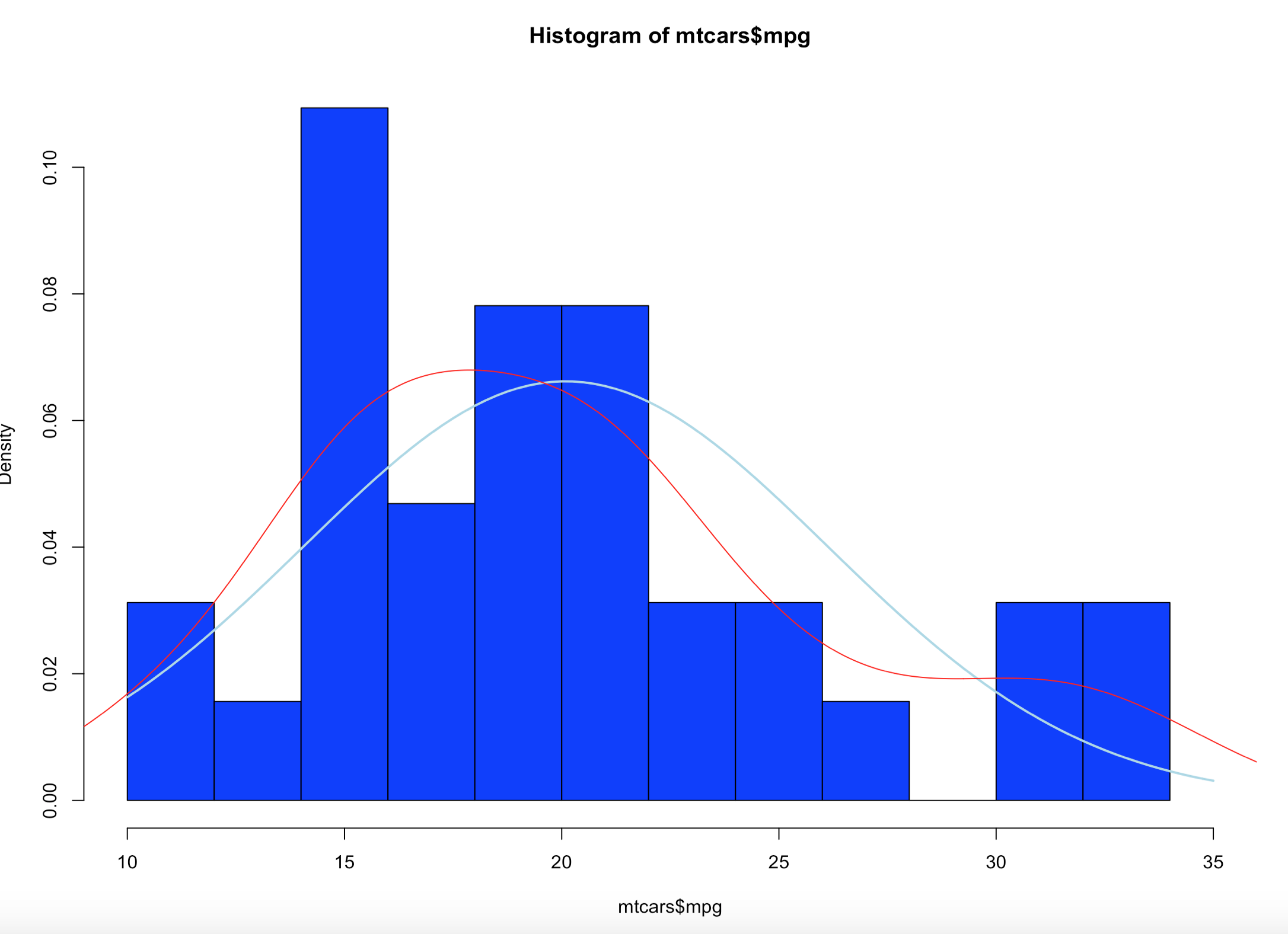
hist(mtcars$mpg,col="blue",breaks=15,freq=FALSE,xlim=c(10,35))

curve(dnorm(x, mean=mean(mtcars$mpg), sd=sd(mtcars$mpg)), col="lightblue",add=TRUE, lwd=2)
Brace yourself, i am going to use as few effective words as possible to describe what curve() and dnorm() did. Looking at at the blue line; what we have now is a PDF, probability density function line. What this means is, since the norm took in the standard deviation and the mean it creates a line density line to try an predict where a new piece of incoming data is likely to fall.

Add a line
lines(density(mtcars$mpg),col="red")
Looking at the red line, this is a kernel density estimate plot layer over the histogram, this basically smoothes the da based on the sample provided. We may get deeper into this way later, as this is pretty advanced. Bu notice how it models the underlying data.
Lets add a mean line in Pink
abline(v = mean(mtcars$mpg),col = "pink",lwd = 3)
The mean as you will recall is the average of the values in mtcars$mpg.
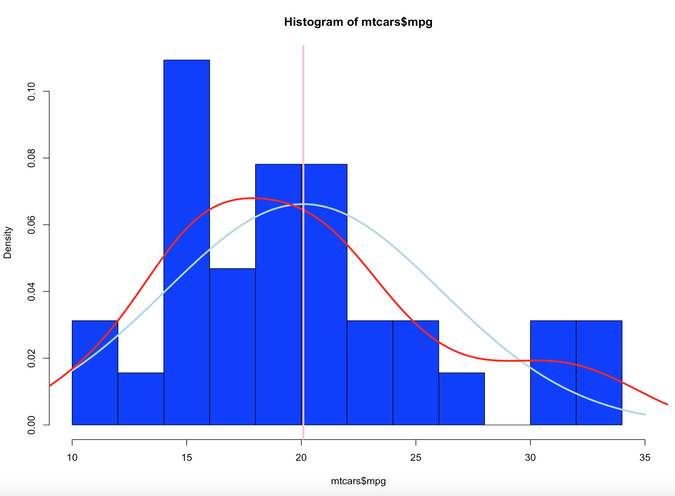
Much more on this very soon, this si a good setup for normal distribution, and the empirical rule.
Shep