In the ongoing visualization show and tell scatterplots have come up next on my list. As I write this blog I try very hard to check and double check my knowledge and methods, I usually have a dataset or two in mind long before I get to the point I want to write about it. This time, I wanted to use the mtcars dataset to play around with the dataset and run a line through the scatter plot to show a trend, lo and behold its already been done to the exact spec I was thinking of doing. Truth be told i am not the first to do any of this, google is your friend when learning R.
So with that, I will do one set with mtcars and send you to Quick-R Scatterplots for the rest. Be careful of some of the visualizations, while nothing will stop you from creating a 3d spinning scatter plot, it is considered chart junk and there is a special website for people who create those are honored. I bet you didn’t know there was a “wtf” domain did you?
I did run into an interesting issue though that I will discuss today, it is a leap ahead, but it is important.
But, lets get some scatterplot going on first.
Below we have loaded the mtcars dataset, and run an attach(). Attach() gives the ability to access the variables/columns of the dataset without having to reference the dataset name. So, instead of mtcars$cyl we can just reference cyl in functions after the attach. It has down sides, so be careful, sort of like a global anything in programming.
data(mtcars)
mtcars
attach(mtcars)
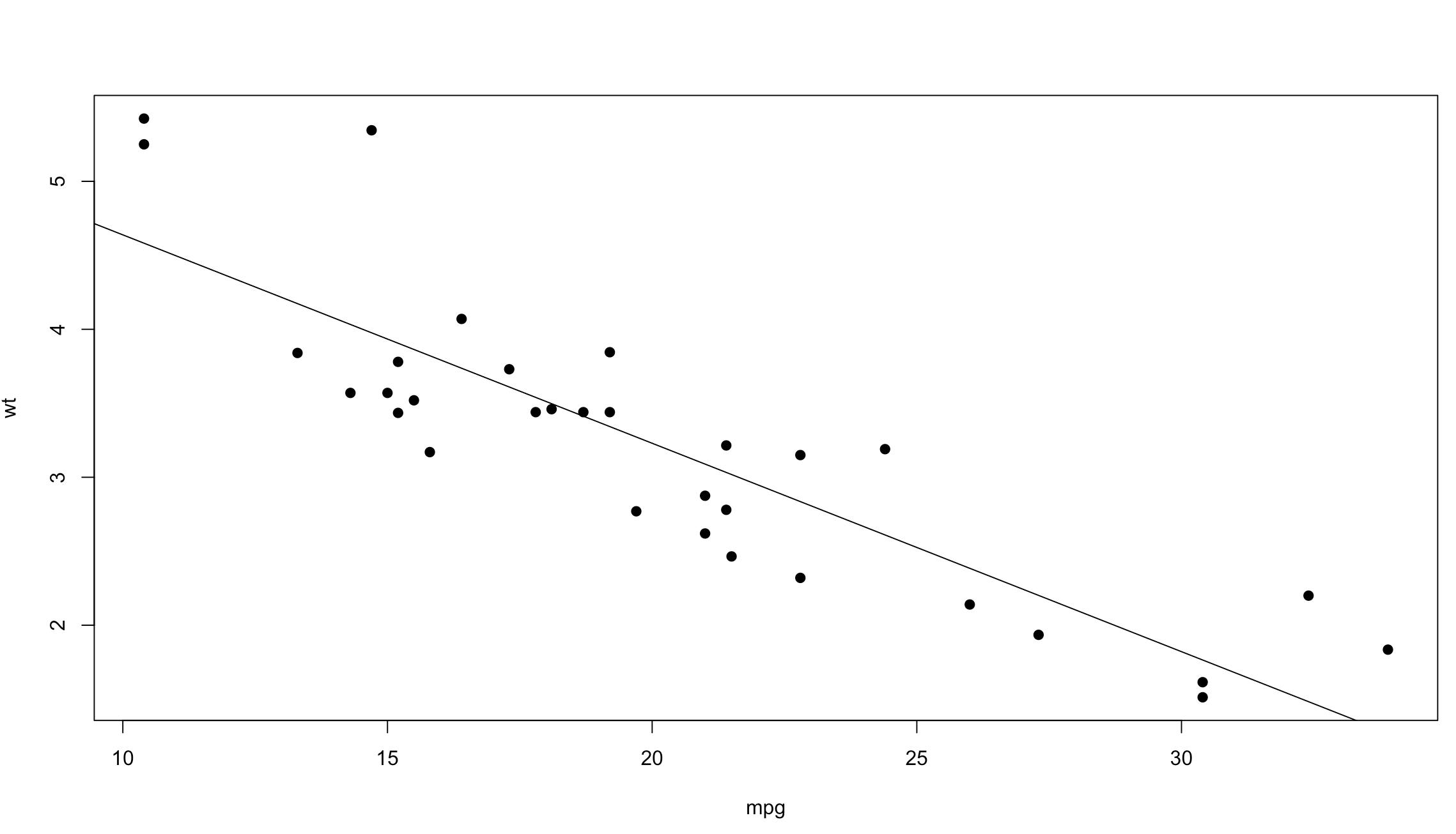
plot(mpg,wt)
With the scatterplot we have two dimensions of data, on the left is the y axis, the weight of the vehicle in thousands of pounds, and on the bottom is the x axis, mpg or miles per gallon.

That was cool, no? Lets add “pch=19” to the next plot to make the dots a bit more visible, and add a line through the data. Abline() draws a straight line through the plot using intercept and slope, we can get the intercept and slope by passing the wt and mpg into a linear model function called lm(). Run lm(wt ~ mpg) by itself and see what you get. Make sure mpg and wt are in the order specified below, “mpg, wt” for the plot and wt~mpg for the lm function. if you dig into the lm() function you will see that we are passing in just a formula of “wt ~ mpg”, from the R documentation for lm() y must be first which is the response variable. Much, Much more on this later, just know for now, y must be first when using lm(), not x.
data(mtcars)
mtcars
attach(mtcars)

plot(mpg,wt,pch=19)
abline(lm(wt ~ mpg))
So, using our scatterplot and the lm function it would appear that as weight increases mpg decreases.
Well thats all pretty cool, but a straight line through my data gives me an idea of the trend but can be misleading if the data is wiggly in the scatter plot, or appears not to be trending.
plot(hp, mpg, main="Scatterplot Example",
     xlab="Horsepower", ylab="MPG", pch=19)
lines(lowess(hp,mpg), col="blue")
Using the lines() and “lowess” option you can see that the line is a little more in tune with the trend of the data. LOWESS is locally weighted scatterplot smoothing. This is much more than just intercept and slope. Depending on the package you are using, there is more than one way to get a line to fit the data.

Lets have a little fun. Hopefully you have played with the mtcars dataset a little bit and maybe even tried out some of the other base R datasets, or loaded your own. The best way to engage in topics like this is to use a dataset you have some passion or curiosity about.
I have a dataset for you on my github site, FL-Median-Population.
This dataset contains the following;
region – County name
CountyFipsCode – The Federal Information Processing Standard code the uniquely identifies the county.
population – American Community Survey estimated population
CollegeDegree – percentage of residents that have completed at least an undergraduate degree.
College – this is the sum of CollegeDegree percentage and the completed some college percentage.
We will be using the xyplot from the lattice package, and the dataset listed above, be sure to change the file location two where every you put it, or use setwd to set your working directory. For this we will start with just the population and median income.
install.packages("lattice")
library(lattice)

florida <- read.csv("/Blog/FloridaData/FL-Median-Population.csv")

xyplot(population ~ MedianIncome,
       data=florida,
       pch=19,
       main="Population vs Income",
       xlab="Median Income",
       ylab = "Populaton")
Hopefully your plot looks a little bit, or exactly like this one. I think this is a good example because it is an imperfect sample. Hopefully on a good day you will get something more like this, and not complete randomness. One point to notice right away is there is one dot way out of range of the rest of the dots at the top of population. Not hard to figure out that is probably the county that Miami resides in, Miami-Dade, and then four other counties coming in at over a population of 1 million. You will also notice there is one county way off to the right in median income, that is St Johns county, which is where the city of Jacksonville is located. Now the median income of Jacksonville is lower than the median income of the county, so what could be going on there?
Hmmm, this just raises more questions, it just so happens, with a population of about 27,000 Ponte Vedra Beach has a median income of $116,000 according to wikipedia, so this one city is dragging the average for the entire county of 220,257 up pretty significantly compared to other counties. So, the with the population of Miami-Dade and the median income of St. Johns being far away from the rest of the data, these are what we call outliers. For now we are going to leave them in, in the next couple of blogs i will demonstrate a method for dealing with outliers. Clearly one like the county of St. Johns will need to be handled eventually.
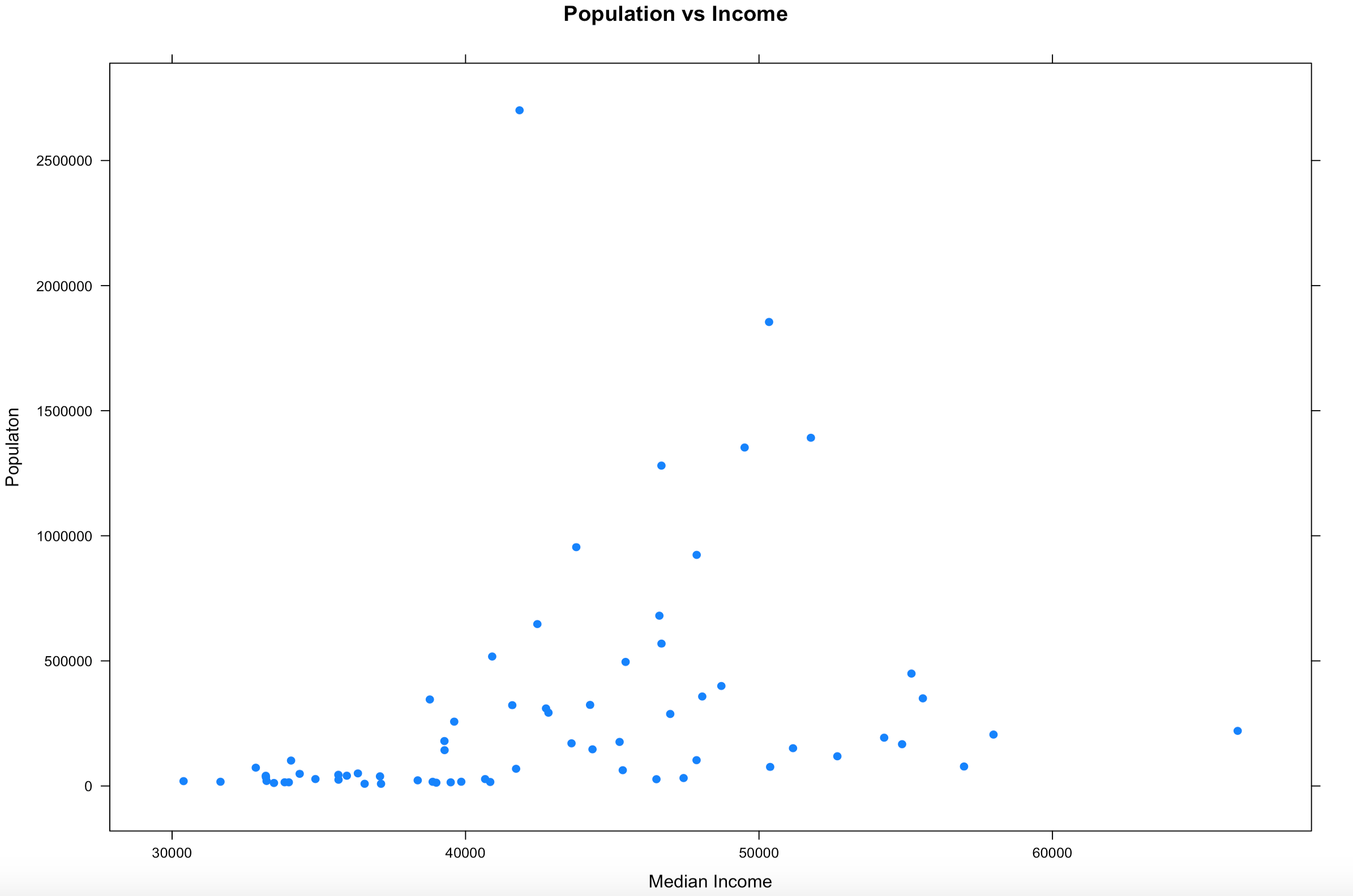
So from looking at the scatter plot, we can kind of make out a general direction of the relationship of income to population, but it is sort of vague. In cases like this there are a few things to do.
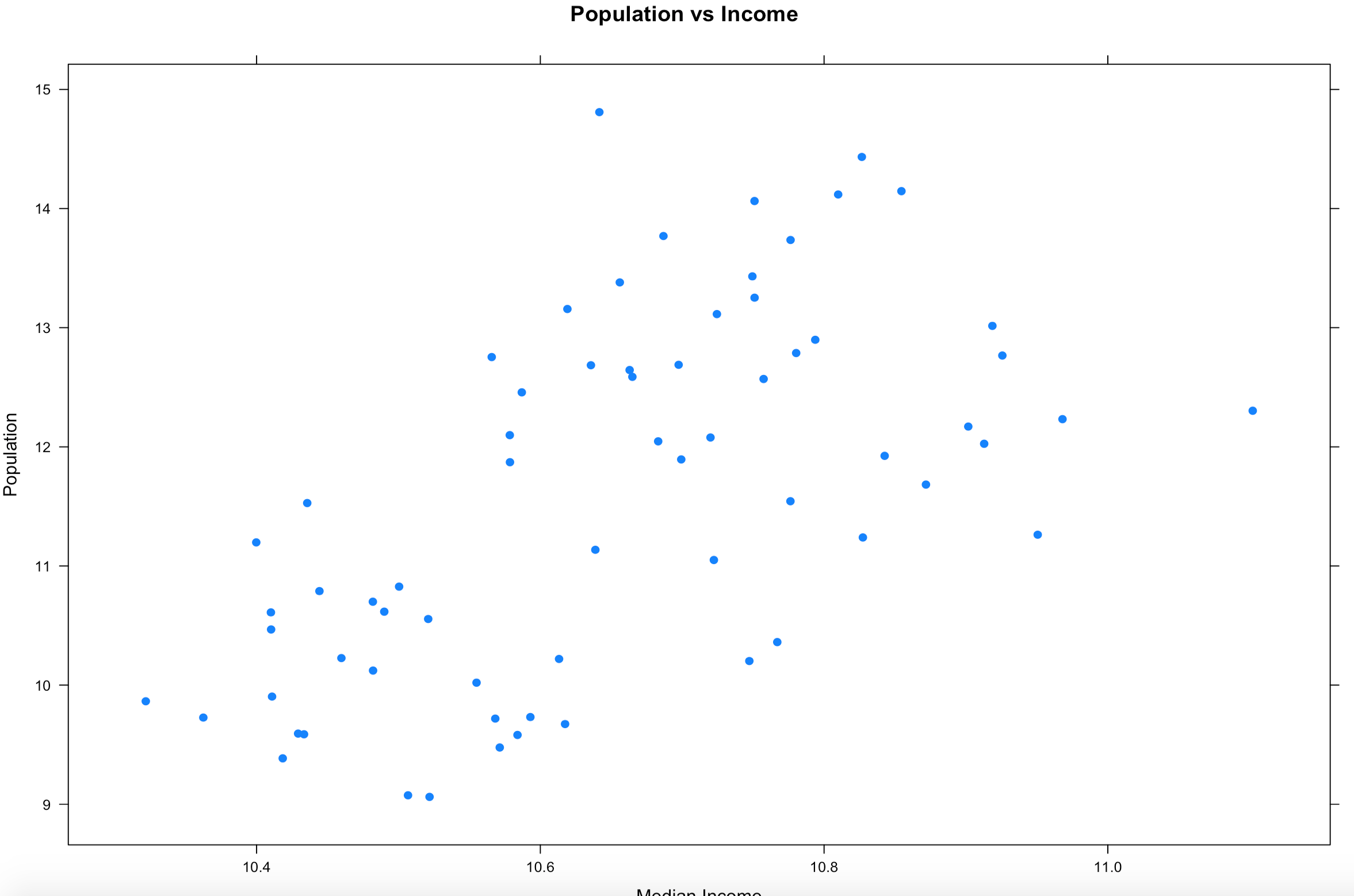
1. When your data looks like it has gone to crazy town, try applying a transformation function for a better graphical representation. This will change the x/y scale, but will still represent the trend of the data. More on log transforms here.
xyplot(log(population) ~ log(MedianIncome),
       data=florida,
       main="Population vs Income",
       xlab="Median Income",
       ylab = "Population",
       pch=19)
2. Draw a linear regression line through it so see if there is a trend. We will get into lm() later, but it takes the (y ~ x) as model input and returns an intercept and slope, remember algebra? 🙂
There is more than one way to do this, xyplot uses the panel function, the much lengthier syntax.
xyplot(log(population) ~ log(MedianIncome),
       data=florida,
       main="Population vs Income",
       xlab="Median Income",
       ylab = "Population",
       panel = function(x, y, ...) {
       panel.xyplot(x, y, ...)
       panel.abline(lm(y~x), col='red',lwd=2)},
       pch=19)
##
## OR
##

plot(log(florida$MedianIncome),log(florida$population),pch=19)
abline(lm(log(florida$population) ~ log(florida$MedianIncome)))
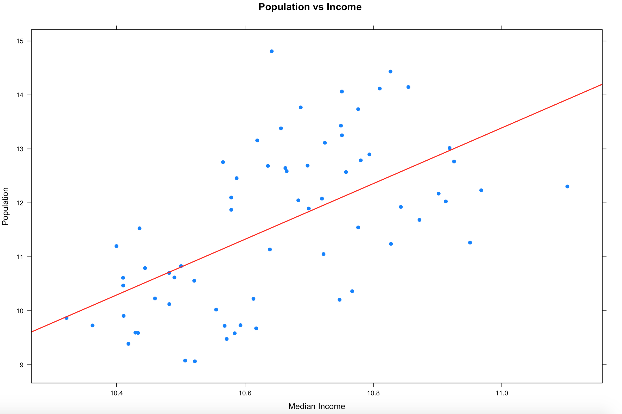
3. In the previous sample we just used a lm, straight line, slope and intercept to run a line through the data, that alone does show a trend. Even if you remove the log function you still seen upward trend of greater population seems to indicate greater income.
So lets try the LOWESS again, this time with xyplot. The type parameter below is using a "p" parameter, this is the LOWESS (locally weighted scatterplot smoothing), it will take our bumpy data and smooth the line to the data. You can read up on it, we will be hitting it thoroughly later on.
xyplot(log(population) ~ log(MedianIncome),
       data=florida,
       main="Population vs Income",
       xlab="Median Income",
       ylab = "Population",
       type = c("p", "smooth"), col.line = "red", lwd = 2,
       pch=19)
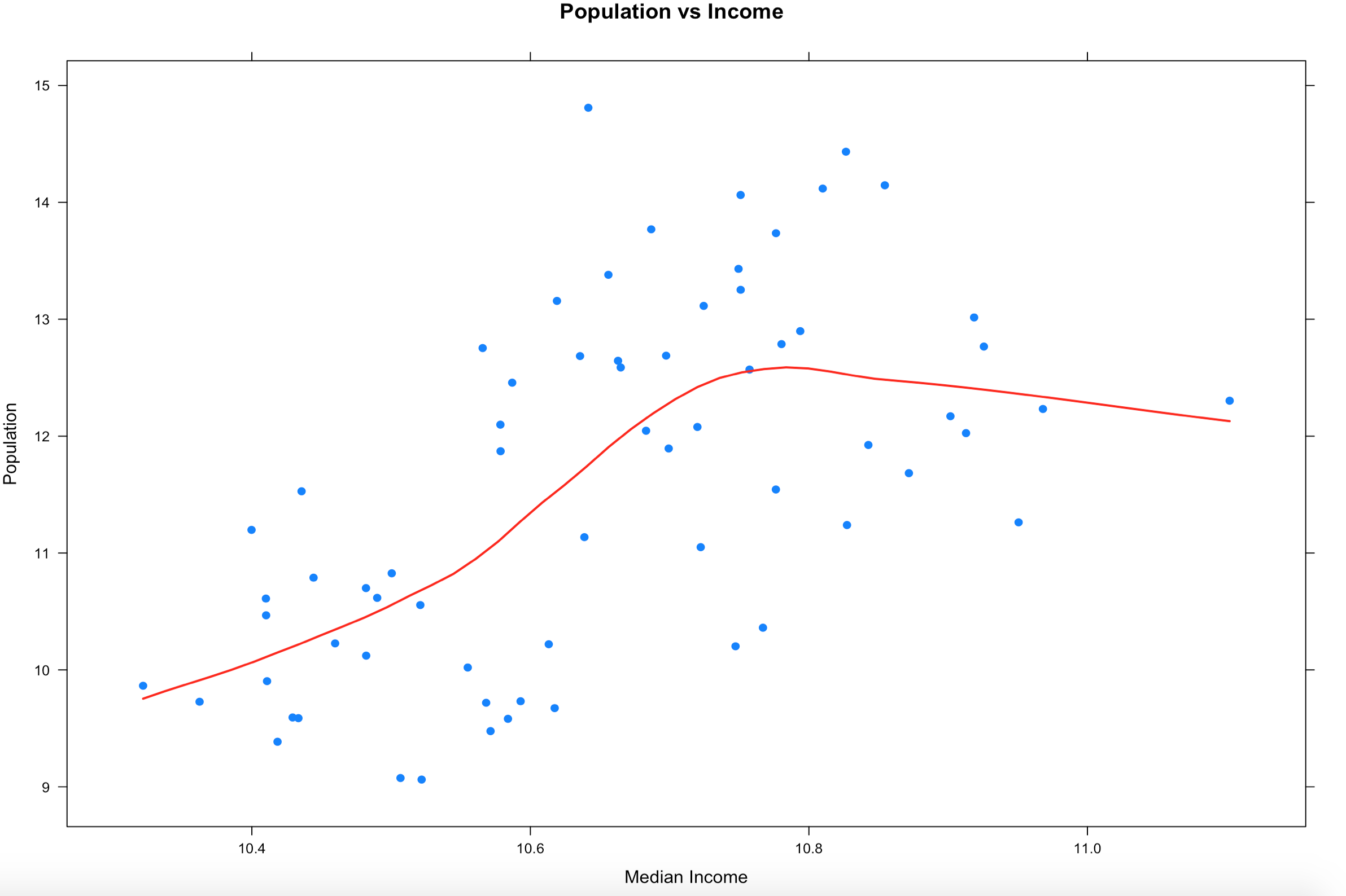
One thing appear to be somewhat clear from this, as the population of the county increases, the income does increase to a point hen it seems to stabilize. We will revisit this once we learn how to deal with outliers and see if it changes the trend.
There are a couple more columns in the Florida data provided that you can try on your own, see if you can visually show a relationship between college and income, or even college and population. Do more rural counties have more or less college educated population?