More variables! For this one we are going to add all of the variables in their correct form in the data frame as qualitative or quantitative.

If you starting with this post, lets get the data loaded up, fix the column names, convert factors to a type of factor, and create a column for out non imperial friends so they can understand the mpg thing.

# Load the data
data(mtcars)

# Create a Liters per 100k column
mtcars$lp100k <- (100 * 3.785) / (1.609 * mtcars$mpg)

#rename the columns to something slightly more meaningful
names(mtcars)[2]<-paste("Cylinders")
names(mtcars)[3]<-paste("Displacement")
names(mtcars)[4]<-paste("Horsepower")
names(mtcars)[5]<-paste("RearAxleRatio")
names(mtcars)[6]<-paste("Weight")
names(mtcars)[7]<-paste("QuarterMile")
names(mtcars)[8]<-paste("VSengine")
names(mtcars)[9]<-paste("TransmissionAM")
names(mtcars)[10]<-paste("Gears")
names(mtcars)[11]<-paste("Carburetors")

#fix the row names, i want them to be a column  
mtcars$Model <- row.names(mtcars)
row.names(mtcars) <- NULL
names(mtcars)

#create factors
ColNames <- c("Cylinders","VSengine","TransmissionAM","Gears","Carburetors")
mtcars[ColNames] <- lapply(mtcars[ColNames], factor)

So the data engineering, though minor, is done, lets go ahead and created a model with everything and see what happens. You can, if you like, run some analysis on all of the new columns using plot to see how the data looks, and if their appear to be any relationships.

The following is a bit ridiculous and i would only advise running this on smaller datasets, but its fun. On my machine, 2+ year old Mac takes about 1 minute run, so be patient, it will give you status update in the console as it runs. I will let you review it on your own instead of putting the graphic here. Also note that if you run this before the categorical columns are converted to factors you will get correlations for those columns.

library(ggplot2)
library(GGally)
ggpairs(mtcars[1:12], aes(alpha = 0.5))

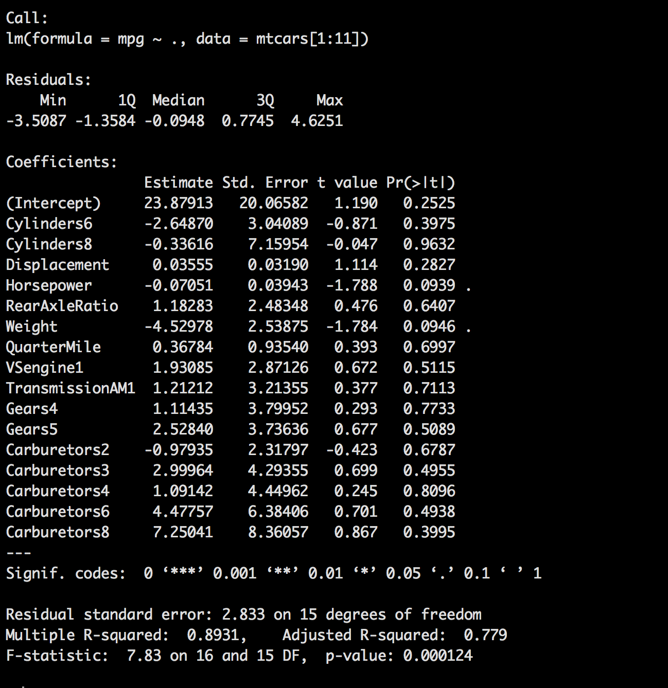
In the last post we left off at mtcars.7, so we will start with mtcars.8 to load our new model. There are a couple of ways to pass the column names into the model, we need the following in the model "mpg", "Cylinders", "Displacement", "Horsepower", "RearAxleRatio", "Weight", "QuarterMile", "VSengine", "TransmissionAM", "Gears", "Carburetors", so we can list them individual as we have in the past, or cheat by slicing the dataframe. If we did not have the slice it would include model and lp100k which we do not want for this.

# The dot will pass everything columns 1-11 to the model.  

mtcars.8 <- lm(mpg ~ ., data=mtcars[1:11])
summary(mtcars.8)

#Or, 

#mtcars.8 <- lm(mpg ~ Cylinders+ Displacement+ Horsepower+ RearAxleRatio+ Weight+ QuarterMile+ VSengine+ TransmissionAM+ Gears+ Carburetors, data=mtcars)

One thing you will notice pretty quickly is using our standard of < .05 of a p-value, that nothing is significant. While we know for a fact that with less variables we do have some significant variables.

We demonstrated a couple of posts ago that adding and subtracting a variable one at a time will change the model, sometimes for the better or the worse and that is what we will do here, but instead of creating each model plus or minus one variable we will let the software do it for us. Stepwise regression which is a form of subset selection. ISLR, page 204 defines Subset Selection as "This approach involves identifying a subset of the p predictors that we believe to be related to the response. We then fit a model using least squares on the reduced set of variables.", and i really like that definition.

Two main forms of stepwise regression, forward stepwise selection and backward stepwise selection.

Forward Stepwise selection starts with a model containing no predictors and then adds the predictors to the model one at a time. ISLR page 207 demonstrates the forward stepwise model as a variable is added and kept if it has the lowest RSS and highest R-squared.

So lets try it!

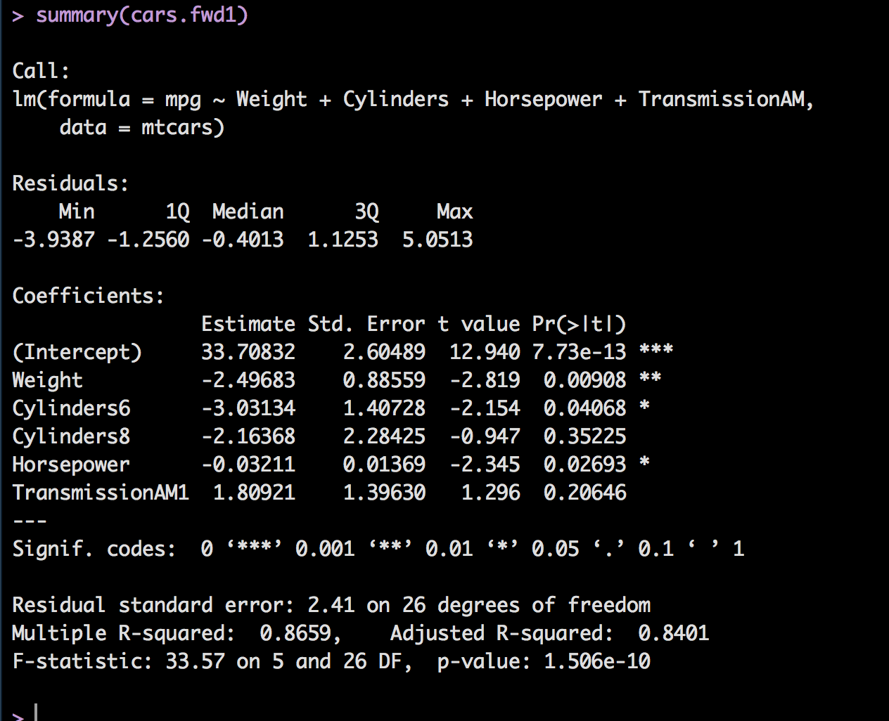
First we will try out a Forward Stepwise, scope is required and you will need to pass in each variable you want to be tested. Just as a normal regression the best and final model will be stored in cars.fwd1 which you can run summary on to get the results.

##stepwise regression forward
cars.fwd1 <- step(lm(mpg~1,data=mtcars), direction = "forward", 
                  scope=(~Cylinders+ Displacement+ Horsepower+ RearAxleRatio+ Weight+ QuarterMile+ VSengine+ TransmissionAM+ Gears+ Carburetors))
summary(cars.fwd1)

That was easy, and fast! Also notice that is kept a couple of variables that had a p-value > .05. This is because the benefit of the variable being there outweighed removing it, lower r-square and likely higher residual error. Also reember that since we are using indicator variables, or dummy variables like Cylinders and transmission, if you keep one of the indicators you ahve to keep them all, they are still on column of data in the original dataset.

So that was fun, what about backward stepwise? The syntax is slightly different for backward stepwise, no scope command and you pass everything into lm(). Same principle as forward but in reverse.

cars.back1 <- step(lm(mpg ~ Cylinders+ Displacement+ Horsepower+ RearAxleRatio+ Weight+ QuarterMile+ VSengine+ TransmissionAM+ Gears+ Carburetors,data=mtcars), direction = "backward")
summary(cars.back1)

In this case, which does not happen every time, you can see that the same model was generated for forward and backwards. So it is reasonable to assume based on the data we have, this is the best we can do.

All of the code to date for Multiple lm can be found here.